1 Geographic data in Python

1.1 Introduction

This chapter outlines two fundamental geographic data models — vector and raster — and introduces the main Python packages for working with them. Before demonstrating their implementation in Python, we will introduce the theory behind each data model and the disciplines in which they predominate.

The vector data model (sec-vector-data) represents the world using points, lines, and polygons. These have discrete, well-defined borders, meaning that vector datasets usually have a high level of precision (but not necessarily accuracy). The raster data model (sec-raster-data), on the other hand, divides the surface up into cells of constant size. Raster datasets are the basis of background images used in web-mapping and have been a vital source of geographic data since the origins of aerial photography and satellite-based remote sensing devices. Rasters aggregate spatially specific features to a given resolution, meaning that they are consistent over space and scalable, with many worldwide raster datasets available.

Which to use? The answer likely depends on your domain of application, and the datasets you have access to:

Vector datasets and methods dominate the social sciences because human settlements and and processes (e.g., transport infrastructure) tend to have discrete borders
Raster datasets and methods dominate many environmental sciences because of the reliance on remote sensing data

Python has strong support for both data models. We will focus on shapely and geopandas for working with geograpic vector data, and rasterio for working with rasters.

shapely is a “low-level” package for working with individual vector geometry objects. geopandas is a “high-level” package for working with geometry columns (GeoSeries objects), which internally contain shapely geometries, and with vector layers (GeoDataFrame objects). The geopandas ecosystem provides a comprehensive approach for working with vector layers in Python, with many packages building on it.

There are several partially overlapping packages for working with raster data, each with its own advantages and disadvantages. In this book, we focus on the most prominent one: rasterio, which represents “simple” raster datasets with a combination of a numpy array, and a metadata object (dict) providing geographic metadata such as the coordinate system. xarray is a notable alternative to rasterio not covered in this book which uses native xarray.Dataset and xarray.DataArray classes to effectively represent complex raster datasets such as ‘NetCDF’ files with multiple bands and metadata.

There is much overlap in some fields and raster and vector datasets can be used together: ecologists and demographers, for example, commonly use both vector and raster data. Furthermore, it is possible to convert between the two forms (see sec-raster-vector). Whether your work involves more use of vector or raster datasets, it is worth understanding the underlying data models before using them, as discussed in subsequent chapters.

1.2 Vector data

The geographic vector data model is based on points located within a coordinate reference system (CRS). Points can represent self-standing features (e.g., the location of a bus stop), or they can be linked together to form more complex geometries such as lines and polygons. Most point geometries contain only two dimensions (3-dimensional CRSs may contain an additional \(z\) value, typically representing height above sea level).

In this system, London, for example, can be represented by the coordinates (-0.1,51.5). This means that its location is -0.1 degrees east and 51.5 degrees north of the origin. The origin, in this case, is at 0 degrees longitude (a prime meridian located at Greenwich) and 0 degrees latitude (the Equator) in a geographic (‘lon/lat’) CRS (Figure fig-vector-london, left panel). The same point could also be approximated in a projected CRS with ‘Easting/Northing’ values of (530000,180000) in the British National Grid, meaning that London is located 530 \(km\) East and 180 \(km\) North of the origin of the CRS (Figure fig-vector-london, right panel). The location of National Grid’s origin, in the sea beyond South West Peninsular, ensures that most locations in the UK have positive Easting and Northing values.

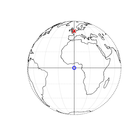
Figure 1.1: Illustration of vector (point) data in which location of London (the red X) is represented with reference to an origin (the blue circle). The left plot represents a geographic CRS with an origin at 0° longitude and latitude. The right plot represents a projected CRS with an origin located in the sea west of the South West Peninsula.

There is more to CRSs, as described in sec-coordinate-reference-systems-intro and sec-reproj-geo-data but, for the purposes of this section, it is sufficient to know that coordinates consist of two numbers representing the distance from an origin, usually in \(x\) and \(y\) dimensions.

geopandas (Bossche et al. 2023) provides classes for geographic vector data and a consistent command-line interface for reproducible geographic data analysis in Python. It also provides an interface to three mature libraries for geocomputation which, in combination, represent a strong foundation on which many geographic applications are built (including QGIS and R’s spatial ecosystem):

GDAL, for reading, writing, and manipulating a wide range of geographic data formats, covered in sec-read-write
PROJ, a powerful library for coordinate system transformations, which underlies the content covered in sec-reproj-geo-data
GEOS, a planar geometry engine for operations such as calculating buffers and centroids on data with a projected CRS, covered in sec-geometric-operations

Tight integration with these geographic libraries makes reproducible geocomputation possible: an advantage of using a higher level language such as Python to access these libraries is that you do not need to know the intricacies of the low level components, enabling focus on the methods rather than the implementation.

1.2.1 Vector data classes

The main classes for working with geographic vector data in Python are hierarchical, meaning the highest level ‘vector layer’ class is composed of simpler ‘geometry column’ and individual ‘geometry’ components. This section introduces them in order, starting with the highest level class. For many applications, the high level vector layer class, which are essentially a data frame with geometry columns, are all that’s needed. However, it’s important to understand the structure of vector geographic objects and their component pieces for more advanced applications. The three main vector geographic data classes in Python are:

GeoDataFrame, a class representing vector layers, with a geometry column (class GeoSeries) as one of the columns
GeoSeries, a class that is used to represent the geometry column in GeoDataFrame objects
shapely geometry objects which represent individual geometries, such as a point or a polygon in GeoSeries objects

The first two classes (GeoDataFrame and GeoSeries) are defined in geopandas. The third class is defined in the shapely package, which deals with individual geometries, and is a main dependency of the geopandas package.

1.2.2 Vector layers

The most commonly used geographic vector data structure is the vector layer. There are several approaches for working with vector layers in Python, ranging from low-level packages (e.g., osgeo, fiona) to the relatively high-level geopandas package that is the focus of this section. Before writing and running code for creating and working with geographic vector objects, we need to import geopandas (by convention as gpd for more concise code) and shapely.

import pandas as pd
import shapely
import geopandas as gpd

We also limit the maximum number of printed rows to six, to save space, using the 'display.max_rows' option of pandas.

pd.set_option('display.max_rows', 6)

Projects often start by importing an existing vector layer saved as a GeoPackage (.gpkg) file, an ESRI Shapefile (.shp), or other geographic file format. The function gpd.read_file imports a GeoPackage file named world.gpkg located in the data directory of Python’s working directory into a GeoDataFrame named gdf.

gdf = gpd.read_file('data/world.gpkg')

The result is an object of type (class) GeoDataFrame with 177 rows (features) and 11 columns, as shown in the output of the following code:

type(gdf)

geopandas.geodataframe.GeoDataFrame

gdf.shape

(177, 11)

The GeoDataFrame class is an extension of the DataFrame class from the popular pandas package (McKinney 2010). This means we can treat non-spatial attributes from a vector layer as a table, and process them using the ordinary, i.e., non-spatial, established function methods. For example, standard data frame subsetting methods can be used. The code below creates a subset of the gdf dataset containing only the country name and the geometry.

gdf = gdf[['name_long', 'geometry']]
gdf

	name_long	geometry
0	Fiji	MULTIPOLYGON (((-180 -16.55522,...
1	Tanzania	MULTIPOLYGON (((33.90371 -0.95,...
2	Western Sahara	MULTIPOLYGON (((-8.66559 27.656...
...	...	...
174	Kosovo	MULTIPOLYGON (((20.59025 41.855...
175	Trinidad and Tobago	MULTIPOLYGON (((-61.68 10.76, -...
176	South Sudan	MULTIPOLYGON (((30.83385 3.5091...

177 rows × 2 columns

The following expression creates a subdataset based on a condition, such as equality of the value in the 'name_long' column to the string 'Egypt'.

gdf[gdf['name_long'] == 'Egypt']

	name_long	geometry
163	Egypt	MULTIPOLYGON (((36.86623 22, 36...

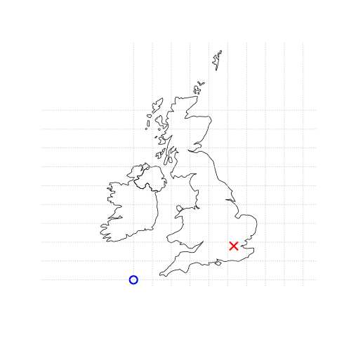
Finally, to get a sense of the spatial component of the vector layer, it can be plotted using the .plot method (Figure fig-gdf-plot).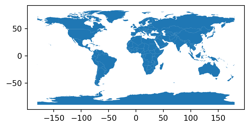

gdf.plot();

Figure 1.2: Basic plot of a `GeoDataFrame`

Interactive maps of GeoDataFrame objects can be created with the .explore method, as illustrated in Figure fig-gdf-explore which was created with the following command:

gdf.explore()

Make this Notebook Trusted to load map: File -> Trust Notebook

Figure 1.3: Basic interactive map with .explore

A subset of the data can be also plotted in a similar fashion.

gdf[gdf['name_long'] == 'Egypt'].explore()

Make this Notebook Trusted to load map: File -> Trust Notebook

Figure 1.4: Interactive map of a GeoDataFrame subset

1.2.3 Geometry columns

The geometry column of class GeoSeries is an essential column in a GeoDataFrame. It contains the geometric part of the vector layer, and is the basis for all spatial operations. This column can be accessed by name, which typically (e.g., when reading from a file) is 'geometry', as in gdf['geometry']. However, the recommendation is to use the fixed .geometry property, which refers to the geometry column regardless whether its name is 'geometry' or not. In the case of the gdf object, the geometry column contains 'MultiPolygon's associated with each country.

gdf.geometry

0      MULTIPOLYGON (((-180 -16.55522,...
1      MULTIPOLYGON (((33.90371 -0.95,...
2      MULTIPOLYGON (((-8.66559 27.656...
                      ...                
174    MULTIPOLYGON (((20.59025 41.855...
175    MULTIPOLYGON (((-61.68 10.76, -...
176    MULTIPOLYGON (((30.83385 3.5091...
Name: geometry, Length: 177, dtype: geometry

The geometry column also contains the spatial reference information, if any (also accessible with the shortcut gdf.crs).

gdf.geometry.crs

<Geographic 2D CRS: EPSG:4326>
Name: WGS 84
Axis Info [ellipsoidal]:
- Lat[north]: Geodetic latitude (degree)
- Lon[east]: Geodetic longitude (degree)
Area of Use:
- name: World.
- bounds: (-180.0, -90.0, 180.0, 90.0)
Datum: World Geodetic System 1984 ensemble
- Ellipsoid: WGS 84
- Prime Meridian: Greenwich

Many geometry operations, such as calculating the centroid, buffer, or bounding box of each feature, involve just the geometry. Applying this type of operation on a GeoDataFrame is therefore basically a shortcut to applying it on the GeoSeries object in the geometry column. For example, the two following commands return exactly the same result, a GeoSeries with country bounding box polygons (using the .envelope method).

gdf.envelope

0      POLYGON ((-180 -18.28799, 179.9...
1      POLYGON ((29.34 -11.72094, 40.3...
2      POLYGON ((-17.06342 20.99975, -...
                      ...                
174    POLYGON ((20.0707 41.84711, 21....
175    POLYGON ((-61.95 10, -60.895 10...
176    POLYGON ((23.88698 3.50917, 35....
Length: 177, dtype: geometry

gdf.geometry.envelope

0      POLYGON ((-180 -18.28799, 179.9...
1      POLYGON ((29.34 -11.72094, 40.3...
2      POLYGON ((-17.06342 20.99975, -...
                      ...                
174    POLYGON ((20.0707 41.84711, 21....
175    POLYGON ((-61.95 10, -60.895 10...
176    POLYGON ((23.88698 3.50917, 35....
Length: 177, dtype: geometry

Note that .envelope, and other similar operators in geopandas such as .centroid (sec-centroids), .buffer (sec-buffers) or .convex_hull, return only the geometry (i.e., a GeoSeries), not a GeoDataFrame with the original attribute data. In case we want the latter, we can create a copy of the GeoDataFrame and then “overwrite” its geometry (or, we can overwrite the geometries directly in case we do not need the original ones, as in gdf.geometry=gdf.envelope).

gdf2 = gdf.copy()
gdf2.geometry = gdf.envelope
gdf2

	name_long	geometry
0	Fiji	POLYGON ((-180 -18.28799, 179.9...
1	Tanzania	POLYGON ((29.34 -11.72094, 40.3...
2	Western Sahara	POLYGON ((-17.06342 20.99975, -...
...	...	...
174	Kosovo	POLYGON ((20.0707 41.84711, 21....
175	Trinidad and Tobago	POLYGON ((-61.95 10, -60.895 10...
176	South Sudan	POLYGON ((23.88698 3.50917, 35....

177 rows × 2 columns

Another useful property of the geometry column is the geometry type, as shown in the following code. Note that the types of geometries contained in a geometry column (and, thus, a vector layer) are not necessarily the same for every row. It is possible to have multiple geometry types in a single GeoSeries. Accordingly, the .type property returns a Series (with values of type str, i.e., strings), rather than a single value (the same can be done with the shortcut gdf.geom_type).

gdf.geometry.type

0      MultiPolygon
1      MultiPolygon
2      MultiPolygon
           ...     
174    MultiPolygon
175    MultiPolygon
176    MultiPolygon
Length: 177, dtype: object

To summarize the occurrence of different geometry types in a geometry column, we can use the pandas .value_counts method. In this case, we see that the gdf layer contains only 'MultiPolygon' geometries.

gdf.geometry.type.value_counts()

MultiPolygon    177
Name: count, dtype: int64

A GeoDataFrame can also have multiple GeoSeries columns, as demonstrated in the following code section.

gdf['bbox'] = gdf.envelope
gdf['polygon'] = gdf.geometry
gdf

Only one geometry column at a time is “active”, in the sense that it is being accessed in operations involving the geometries (such as .centroid, .crs, etc.). To switch the active geometry column from one GeoSeries column to another, we use .set_geometry. Figure fig-switch-to-centroids and Figure fig-switch-to-polygons shows interactive maps of the gdf layer with the 'bbox' and 'polygon' geometry columns activated, respectively.

gdf = gdf.set_geometry('bbox')
gdf.explore()

Make this Notebook Trusted to load map: File -> Trust Notebook

Figure 1.5: Switching to the 'bbox' geometry column in the world layer, and plotting it

gdf = gdf.set_geometry('polygon')
gdf.explore()

Make this Notebook Trusted to load map: File -> Trust Notebook

Figure 1.6: Switching to the 'polygons' geometry column in the world layer, and plotting it

1.2.4 The Simple Features standard

Geometries are the basic building blocks of vector layers. Although the Simple Features standard defines about 20 types of geometries, we will focus on the seven most commonly used types: POINT, LINESTRING, POLYGON, MULTIPOINT, MULTILINESTRING, MULTIPOLYGON and GEOMETRYCOLLECTION. A useful list of possible geometry types can be found in R’s sf package documentation¹.

Simple feature geometries can be represented by well-known binary (WKB) and well-known text (WKT) encodings. WKB representations are usually hexadecimal strings easily readable for computers, and this is why GIS software and spatial databases use WKB to transfer and store geometry objects. WKT, on the other hand, is a human-readable text markup description of Simple Features. Both formats are exchangeable, and if we present one, we will naturally choose the WKT representation.

The foundation of each geometry type is the point. A point is simply a coordinate in 2D, 3D, or 4D space such as shown in Figure fig-point.

POINT (5 2)

A linestring is a sequence of points with a straight line connecting the points (Figure fig-linestring).

LINESTRING (1 5, 4 4, 4 1, 2 2, 3 2)

A polygon is a sequence of points that form a closed, non-intersecting ring. Closed means that the first and the last point of a polygon have the same coordinates (Figure fig-polygon).

POLYGON ((1 5, 2 2, 4 1, 4 4, 1 5))

So far we have created geometries with only one geometric entity per feature. However, the Simple Features standard allows multiple geometries to exist within a single feature, using “multi” versions of each geometry type, as illustrated in Figure fig-multipoint, Figure fig-multilinestring, and Figure fig-multipolygon1.

MULTIPOINT (5 2, 1 3, 3 4, 3 2)
MULTILINESTRING ((1 5, 4 4, 4 1, 2 2, 3 2), (1 2, 2 4))
MULTIPOLYGON (((1 5, 2 2, 4 1, 4 4, 1 5), (0 2, 1 2, 1 3, 0 3, 0 2)))

Finally, a geometry collection can contain any combination of geometries of the other six types, such as the combination of a multipoint and linestring shown below (Figure fig-geometrycollection).

GEOMETRYCOLLECTION (MULTIPOINT (5 2, 1 3, 3 4, 3 2),
                    LINESTRING (1 5, 4 4, 4 1, 2 2, 3 2))

1.2.5 Geometries

Each element in the geometry column (GeoSeries) is a geometry object of class shapely (Gillies et al. 2007--). For example, here is one specific geometry selected by implicit index (Canada, the 4^th element in gdf’s geometry column).

gdf.geometry.iloc[3]

We can also select a specific geometry based on the 'name_long' attribute (i.e., the 1^st and only element in the subset of gdf where the country name is equal to Egypt):

gdf[gdf['name_long'] == 'Egypt'].geometry.iloc[0]

The shapely package is compatible with the Simple Features standard (sec-simple-features). Accordingly, seven types of geometry types are supported. The following section demonstrates creating a shapely geometry of each type from scratch. In the first example (a 'Point') we show two types of inputs to create a geometry: a list of coordinates or a string in the WKT format. In the examples for the remaining geometries we use the former approach.

Creating a 'Point' geometry from a list of coordinates uses the shapely.Point function in the following expression (Figure fig-point).

point = shapely.Point([5, 2])
point

Figure 1.7: A `Point` geometry (created either from a `list` or WKT)

Alternatively, we can use shapely.from_wkt to transform a WKT string to a shapely geometry object. Here is an example of creating the same 'Point' geometry from WKT (Figure fig-point).

point = shapely.from_wkt('POINT (5 2)')
point

A 'LineString' geometry can be created based on a list of coordinate tuples or lists (Figure fig-linestring).

linestring = shapely.LineString([(1,5), (4,4), (4,1), (2,2), (3,2)])
linestring

Creation of a 'Polygon' geometry is similar, but our first and last coordinate must be the same, to ensure that the polygon is closed. Note that in the following example, there is one list of coordinates that defines the exterior outer hull of the polygon, followed by a list of lists of coordinates that define the holes (if any) in the polygon (Figure fig-polygon).

polygon = shapely.Polygon(
    [(1,5), (2,2), (4,1), (4,4), (1,5)],  ## Exterior
    [[(2,4), (3,4), (3,3), (2,3), (2,4)]]  ## Hole(s)
)
polygon

A 'MultiPoint' geometry is also created from a list of coordinate tuples (Figure fig-multipoint), where each element represents a single point.

multipoint = shapely.MultiPoint([(5,2), (1,3), (3,4), (3,2)])
multipoint

A 'MultiLineString' geometry, on the other hand, has one list of coordinates for each line in the MultiLineString (Figure fig-multilinestring).

multilinestring = shapely.MultiLineString([
    [(1,5), (4,4), (4,1), (2,2), (3,2)],  ## 1st sequence
    [(1,2), (2,4)]  ## 2nd sequence, etc.
])
multilinestring

Figure 1.11: A `MultiLineString` geometry

A 'MultiPolygon' geometry (Figure fig-multipolygon1) is created from a list of Polygon geometries. For example, here we are creating a 'MultiPolygon' with two parts, both without holes.

multipolygon = shapely.MultiPolygon([
    [[(1,5), (2,2), (4,1), (4,4), (1,5)], []],  ## Polygon 1 
    [[(0,2), (1,2), (1,3), (0,3), (0,2)], []]   ## Polygon 2, etc.
])
multipolygon

Since the required input has four hierarchical levels, it may be more clear to create the single-part 'Polygon' geometries in advance, using the respective function (shapely.Polygon), and then pass them to shapely.MultiPolygon (Figure fig-multipolygon1). (The same technique can be used with the other shapely.Multi* functions.)

multipolygon = shapely.MultiPolygon([
    shapely.Polygon([(1,5), (2,2), (4,1), (4,4), (1,5)]),  ## Polygon 1 
    shapely.Polygon([(0,2), (1,2), (1,3), (0,3), (0,2)])   ## Polygon 2, etc.
])
multipolygon

And, finally, a 'GeometryCollection' geometry is a list with one or more of the other six geometry types (Figure fig-geometrycollection):

geometrycollection = shapely.GeometryCollection([multipoint, multilinestring])
geometrycollection

Figure 1.13: A `GeometryCollection` geometry

shapely geometries act as atomic units of vector data, meaning that there is no concept of geometry sets: each operation accepts individual geometry object(s) as input, and returns an individual geometry as output. (The GeoSeries and GeoDataFrame objects, defined in geopandas, are used to deal with sets of shapely geometries, collectively.) For example, the following expression calculates the difference (see sec-clipping) between the buffered (see sec-buffers) multipolygon (using distance of 0.2) and itself (Figure fig-mpol-buffer-difference):

multipolygon.buffer(0.2).difference(multipolygon)

Figure 1.14: The difference between a buffered `MultiPolygon` and itself

As demonstrated in the last few figures, a shapely geometry object is automatically evaluated to a small image of the geometry (when using an interface capable of displaying it, such as Jupyter Notebook). To print the WKT string instead, we can use the print function:

print(linestring)

LINESTRING (1 5, 4 4, 4 1, 2 2, 3 2)

Finally, it is important to note that raw coordinates of shapely geometries are accessible through a combination of the .coords, .geoms, .exterior, and .interiors properties (depending on the geometry type). These access methods are helpful when we need to develop our own spatial operators for specific tasks. For example, the following expression returns the list of all coordinates of the polygon geometry exterior:

list(polygon.exterior.coords)

[(1.0, 5.0), (2.0, 2.0), (4.0, 1.0), (4.0, 4.0), (1.0, 5.0)]

Also see sec-type-transformations, where .coords, .geoms, and .exterior are used to transform a given shapely geometry to a different type (e.g., 'Polygon' to 'MultiPoint').

1.2.6 Vector layer from scratch

In the previous sections, we started with a vector layer (GeoDataFrame), from an existing GeoPackage file, and “decomposed” it to extract the geometry column (GeoSeries, sec-geometry-columns) and separate geometries (shapely, see sec-geometries). In this section, we will demonstrate the opposite process, constructing a GeoDataFrame from shapely geometries, combined into a GeoSeries. This will help you better understand the structure of a GeoDataFrame, and may come in handy when you need to programmatically construct simple vector layers, such as a line between two given points.

Vector layers consist of two main parts: geometries and non-geographic attributes. Figure fig-gdf-flow shows how a GeoDataFrame object is created—geometries come from a GeoSeries object (which consists of shapely geometries), while attributes are taken from Series objects.

Figure 1.15: Creating a `GeoDataFrame` from scratch

The final result, a vector layer (GeoDataFrame) is therefore a hierarchical structure (Figure fig-gdf-structure), containing the geometry column (GeoSeries), which in turn contains geometries (shapely). Each of the “internal” components can be accessed, or “extracted”, which is sometimes necessary, as we will see later on.

Figure 1.16: Structure of a `GeoDataFrame`

Non-geographic attributes may represent the name of the feature, and other attributes such as measured values, groups, etc. To illustrate attributes, we will represent a temperature of 25°C in London on June 21st, 2023. This example contains a geometry (the coordinates), and three attributes with three different classes (place name, temperature and date). Objects of class GeoDataFrame represent such data by combining the attributes (Series) with the simple feature geometry column (GeoSeries). First, we create a point geometry, which we know how to do from sec-geometries (Figure fig-point-lnd).

lnd_point = shapely.Point(0.1, 51.5)
lnd_point

Figure 1.17: A `shapely` point representing London

Next, we create a GeoSeries (of length 1), containing the point and a CRS definition, in this case WGS84 (defined using its EPSG code 4326). Also note that the shapely geometries go into a list, to illustrate that there can be more than one geometry unlike in this example.

lnd_geom = gpd.GeoSeries([lnd_point], crs=4326)
lnd_geom

0    POINT (0.1 51.5)
dtype: geometry

Next, we combine the GeoSeries with other attributes into a dict. The geometry column is a GeoSeries, named geometry. The other attributes (if any) may be defined using list or Series objects. Here, for simplicity, we use the list option for defining the three attributes name, temperature, and date. Again, note that the list can be of length >1, in case we are creating a layer with more than one feature (i.e., multiple rows).

lnd_data = {
  'name': ['London'],
  'temperature': [25],
  'date': ['2023-06-21'],
  'geometry': lnd_geom
}

Finally, the dict can be coverted to a GeoDataFrame object, as shown in the following code.

lnd_layer = gpd.GeoDataFrame(lnd_data)
lnd_layer

	name	temperature	date	geometry
0	London	25	2023-06-21	POINT (0.1 51.5)

What just happened? First, the coordinates were used to create the simple feature geometry (shapely). Second, the geometry was converted into a simple feature geometry column (GeoSeries), with a CRS. Third, attributes were combined with GeoSeries. This results in an GeoDataFrame object, named lnd_layer.

To illustrate how does creating a layer with more than one feature looks like, here is an example where we create a layer with two points, London and Paris.

lnd_point = shapely.Point(0.1, 51.5)
paris_point = shapely.Point(2.3, 48.9)
towns_geom = gpd.GeoSeries([lnd_point, paris_point], crs=4326)
towns_data = {
  'name': ['London', 'Paris'],
  'temperature': [25, 27],
  'date': ['2013-06-21', '2013-06-21'],
  'geometry': towns_geom
}
towns_layer = gpd.GeoDataFrame(towns_data)
towns_layer

	name	temperature	date	geometry
0	London	25	2013-06-21	POINT (0.1 51.5)
1	Paris	27	2013-06-21	POINT (2.3 48.9)

Now, we are able to create an interactive map of the towns_layer object (Figure fig-layer-from-scratch-explore). To make the points easier to see, we are customizing a fill color and size (we elaborate on .explore options in sec-interactive-maps).

towns_layer.explore(color='red', marker_kwds={'radius': 10})

Make this Notebook Trusted to load map: File -> Trust Notebook

Figure 1.18: towns_layer, created from scratch, visualized using .explore

A spatial (point) layer can be also created from a DataFrame object (package pandas) that contains columns with coordinates. To demonstrate, we hereby first create a GeoSeries object from the coordinates, and then combine it with the DataFrame to form a GeoDataFrame.

towns_table = pd.DataFrame({
  'name': ['London', 'Paris'],
  'temperature': [25, 27],
  'date': ['2017-06-21', '2017-06-21'],
  'x': [0.1, 2.3],
  'y': [51.5, 48.9]
})
towns_geom = gpd.points_from_xy(towns_table['x'], towns_table['y'])
towns_layer = gpd.GeoDataFrame(towns_table, geometry=towns_geom, crs=4326)

The output gives the same result as previous towns_layer. This approach is particularly useful when we need to read data from a CSV file, e.g., using pd.read_csv, and want to turn the resulting DataFrame into a GeoDataFrame (see another example in sec-spatial-joining).

1.2.7 Derived numeric properties

Vector layers are characterized by two essential derived numeric properties: length (.length)—applicable to lines, and area (.area)—applicable to polygons. Area and length can be calculated for any data structures discussed above, either a shapely geometry, in which case the returned value is a number, or for GeoSeries or DataFrame, in which case the returned value is a numeric Series.

linestring.length

9.39834563766817

multipolygon.area

8.0

gpd.GeoSeries([point, linestring, polygon, multipolygon]).area

0    0.0
1    0.0
2    6.0
3    8.0
dtype: float64

Like all numeric calculations in geopandas, the results assume a planar CRS and are returned in its native units. This means that length and area measurements for geometries in WGS84 (crs=4326) are returned in decimal degrees and essentially meaningless (to see the warning, try running gdf.area).

To obtain meaningful length and area measurements for data in a geographic CRS, the geometries first need to be transformed to a projected CRS (see sec-reprojecting-vector-geometries) applicable to the area of interest. For example, the area of Slovenia can be calculated in the UTM zone 33N CRS (crs=32633). The result is in \(m^2\), the units of the UTM zone 33N CRS.

gdf[gdf['name_long'] == 'Slovenia'].to_crs(32633).area

150    1.910410e+10
dtype: float64

1.3 Raster data

The spatial raster data model represents the world with the continuous grid of cells (often also called pixels; Figure fig-raster-intro-plot1 (A)). This data model often refers to so-called regular grids, in which each cell has the same, constant size—and we will focus only on regular grids in this book. However, several other types of grids exist, including rotated, sheared, rectilinear, and curvilinear grids (see Chapter 1 of Pebesma and Bivand (2022) or Chapter 2 of Tennekes and Nowosad (2022)).

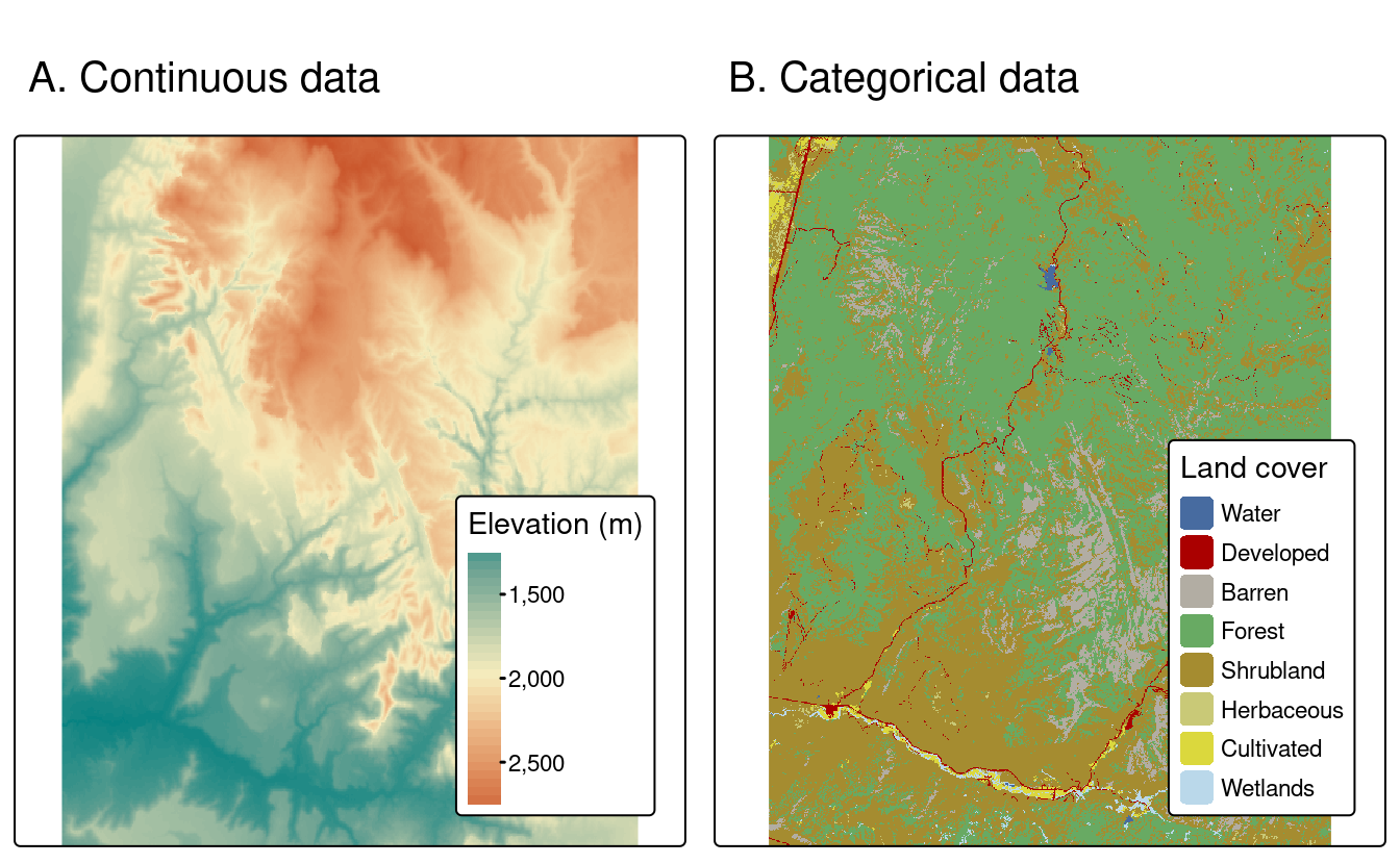
The raster data model usually consists of a raster header (or metadata) and a matrix (with rows and columns) representing equally spaced cells (often also called pixels; Figure fig-raster-intro-plot1 (A)). The raster header defines the coordinate reference system, the the origin and the resolution. The origin (or starting point) is typically the coordinate of the lower-left corner of the matrix. The metadata defines the the origin, and the cell size, i.e., resolution. Combined with the column and row count, the extent can also be derived. The matrix representation avoids storing explicitly the coordinates for the four corner points (in fact it only stores one coordinate, namely the origin) of each cell, as would be the case for rectangular vector polygons. This and map algebra (sec-map-algebra) makes raster processing much more efficient and faster than vector data processing. However, in contrast to vector data, the cell of one raster layer can only hold a single value. The cell values are numeric, representing either a continuous or a categorical variable (Figure fig-raster-intro-plot1 (C)).

Figure 1.19: Raster data types: (A) cell IDs, (B) cell values, (C) a colored raster map

Raster maps usually represent continuous phenomena such as elevation, temperature, population density or spectral data. Discrete features such as soil or land-cover classes can also be represented in the raster data model. Both uses of raster datasets are illustrated in Figure fig-raster-intro-plot2, which shows how the borders of discrete features may become blurred in raster datasets. Depending on the nature of the application, vector representations of discrete features may be more suitable.

Figure 1.20: Examples of continuous and categorical rasters

As mentioned above, working with rasters in Python is less organized around one comprehensive package as compared to the case for vector layers and geopandas. Instead, several packages provide alternative subsets of methods for working with raster data.

The two most notable approaches for working with rasters in Python are provided by rasterio and rioxarray packages. As we will see shortly, they differ in scope and underlying data models. Specifically, rasterio represents rasters as numpy arrays associated with a separate object holding the spatial metadata. The rioxarray package, a wrapper of rasterio, however, represents rasters with xarray “extended” arrays, which are an extension of numpy array designed to hold axis labels and attributes in the same object, together with the array of raster values. Similar approaches are provided by less well-known xarray-spatial and geowombat packages. Comparatively, rasterio is more well-established, but it is more low-level (which has both advantages and distadvantages).

All of the above-mentioned packages, however, are not exhaustive in the same way geopandas is. For example, when working with rasterio, more packages may be needed to accomplish common tasks such as zonal statistics (package rasterstats) or calculating topographic indices (package richdem).

In the following two sections, we introduce rasterio, which is the raster-related package we are going to work with through the rest of the book.

1.3.1 Using rasterio

To work with the rasterio package, we first need to import it. Additionally, as the raster data is stored within numpy arrays, we import the numpy package and make all its functions accessible for effective data manipulation. Finally, we import the rasterio.plot sub-module for its rasterio.plot.show function that allows for quick visualization of rasters.

import numpy as np
import rasterio
import rasterio.plot

Rasters are typically imported from existing files. When working with rasterio, importing a raster is actually a two-step process:

First, we open a raster file “connection” using rasterio.open
Second, we read raster values from the connection using the .read method

This type of separation is analogous to basic Python functions for reading from files, such as open and .readline to read from a text file. The rationale is that we do not always want to read all information from the file into memory, which is particularly important as rasters size can be larger than RAM size. Accordingly, the second step (.read) is selective, meaning that the user can fine tune the subset of values (bands, rows/columns, resolution, etc.) that are actually being read. For example, we may want to read just one raster band rather than reading all bands.

In the first step, we pass a file path to the rasterio.open function to create a DatasetReader file connection, hereby named src. For this example, we use a single-band raster representing elevation in Zion National Park, stored in srtm.tif.

src = rasterio.open('data/srtm.tif')
src

<open DatasetReader name='data/srtm.tif' mode='r'>

To get a first impression of the raster values, we can plot the raster using the rasterio.plot.show function (Figure fig-rasterio-plot):

rasterio.plot.show(src);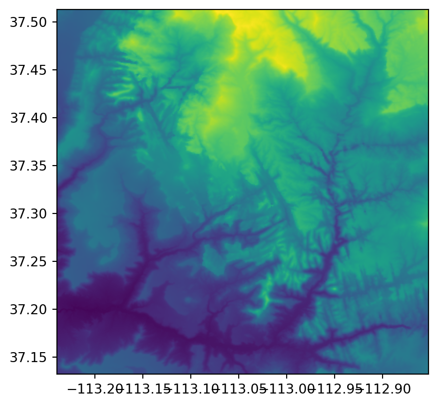

Figure 1.21: Basic plot of a raster, the data are coming from a **rasterio** file connection

The DatasetReader contains the raster metadata, that is, all of the information other than the raster values. Let’s examine it with the .meta property.

src.meta

{'driver': 'GTiff',
 'dtype': 'uint16',
 'nodata': 65535.0,
 'width': 465,
 'height': 457,
 'count': 1,
 'crs': CRS.from_epsg(4326),
 'transform': Affine(0.0008333333332777796, 0.0, -113.23958321278403,
        0.0, -0.0008333333332777843, 37.512916763165805)}

Namely, it allows us to see the following properties, which we will elaborate on below, and in later chapters:

driver—The raster file format (see sec-data-output-raster)
dtype—Data type (see Table tbl-numpy-data-types)
nodata—The value being used as “No Data” flag (see sec-data-output-raster)
Dimensions:
- width—Number of columns
- height—Number of rows
- count—Number of bands
crs—Coordinate reference system (see sec-querying-and-setting-coordinate-systems)
transform—The raster affine transformation matrix

The last item (i.e., transform) deserves more attention. To position a raster in geographical space, in addition to the CRS, we must specify the raster origin (\(x_{min}\), \(y_{max}\)) and resolution (\(delta_{x}\), \(delta_{y}\)). In the transformation matrix notation, assuming a regular grid, these data items are stored as follows:

Affine(delta_x, 0.0, x_min,
       0.0, delta_y, y_max)

Note that, by convention, raster y-axis origin is set to the maximum value (\(y_{max}\)) rather than the minimum, and, accordingly, the y-axis resolution (\(delta_{y}\)) is negative. In other words, since the origin is in the top-left corner, advancing along the y-axis is done through negative steps (downwards).

In the second step, the .read method of the DatasetReader is used to read the actual raster values. Importantly, we can read:

All layers (as in .read())
A particular layer, passing a numeric index (as in .read(1))
A subset of layers, passing a list of indices (as in .read([1,2]))

Note that the layer indices start from 1, contrary to the Python convention of the first index being 0.

The object returned by .read is a numpy array (Harris et al. 2020), with either two or three dimensions:

Three dimensions, when reading more than one layer (e.g., .read() or .read([1,2])). In such case, the dimensions pattern is (layers, rows, columns)
Two dimensions, when reading one specific layer (e.g., .read(1)). In such case, the dimensions pattern is (rows, columns)

Let’s read the first (and only) layer from the srtm.tif raster, using the file connection object src and the .read method.

src.read(1)

array([[1728, 1718, 1715, ..., 2654, 2674, 2685],
       [1737, 1727, 1717, ..., 2649, 2677, 2693],
       [1739, 1734, 1727, ..., 2644, 2672, 2695],
       ...,
       [1326, 1328, 1329, ..., 1777, 1778, 1775],
       [1320, 1323, 1326, ..., 1771, 1770, 1772],
       [1319, 1319, 1322, ..., 1768, 1770, 1772]], dtype=uint16)

The result is a two-dimensional numpy array where each value represents the elevation of the corresponding pixel.

The relation between a rasterio file connection and the derived properties is summarized in Figure fig-rasterio-structure. The file connection (created with rasterio.open) gives access to the two components of raster data: the metadata (via the .meta property) and the values (via the .read method).

Figure 1.22: Creating a `GeoDataFrame` from scratch

1.3.2 Raster from scratch

In this section, we are going to demonstrate the creation of rasters from scratch. We will construct two small rasters, elev and grain, which we will use in examples later in the book. Unlike creating a vector layer (see sec-vector-layer-from-scratch), creating a raster from scratch is rarely needed in practice because aligning a raster with the proper spatial extent is challenging to do programmatically (“georeferencing” tools in GIS software are a better fit for the job). Nevertheless, the examples will be helpful to become more familiar with the rasterio data structures.

Conceptually, a raster is an array combined with georeferencing information, whereas the latter comprises:

A transformation matrix, containing the origin and resolution, thus linking pixel indices with coordinates in a particular coordinate system
A CRS definition, specifying the association of that coordinate system with the surface of the earth (optional)

Therefore, to create a raster, we first need to have an array with the values, and then supplement it with the georeferencing information. Let’s create the arrays elev and grain. The elev array is a \(6 \times 6\) array with sequential values from 1 to 36. It can be created as follows using the np.arange function and .reshape method from numpy.

elev = np.arange(1, 37, dtype=np.uint8).reshape(6, 6)
elev

array([[ 1,  2,  3,  4,  5,  6],
       [ 7,  8,  9, 10, 11, 12],
       [13, 14, 15, 16, 17, 18],
       [19, 20, 21, 22, 23, 24],
       [25, 26, 27, 28, 29, 30],
       [31, 32, 33, 34, 35, 36]], dtype=uint8)

The grain array represents a categorical raster with values 0, 1, 2, corresponding to categories “clay”, “silt”, “sand”, respectively. We will create it from a specific arrangement of pixel values, using numpy’s np.array and .reshape.

v = [
  1, 0, 1, 2, 2, 2, 
  0, 2, 0, 0, 2, 1, 
  0, 2, 2, 0, 0, 2, 
  0, 0, 1, 1, 1, 1, 
  1, 1, 1, 2, 1, 1, 
  2, 1, 2, 2, 0, 2
]
grain = np.array(v, dtype=np.uint8).reshape(6, 6)
grain

array([[1, 0, 1, 2, 2, 2],
       [0, 2, 0, 0, 2, 1],
       [0, 2, 2, 0, 0, 2],
       [0, 0, 1, 1, 1, 1],
       [1, 1, 1, 2, 1, 1],
       [2, 1, 2, 2, 0, 2]], dtype=uint8)

Note that in both cases, we are using the uint8 (unsigned integer in 8 bits, i.e., 0-255) data type, which is sufficient to represent all possible values of the given rasters (see Table tbl-numpy-data-types). This is the recommended approach for a minimal memory footprint.

What is missing now is the georeferencing information (see sec-using-rasterio). In this case, since the rasters are arbitrary, we also set up an arbitrary transformation matrix, where:

The origin (\(x_{min}\), \(y_{max}\)) is at -1.5,1.5
The raster resolution (\(delta_{x}\), \(delta_{y}\)) is 0.5,-0.5

We can add this information using rasterio.transform.from_origin, and specifying west, north, xsize, and ysize parameters. The resulting transformation matrix object is hereby named new_transform.

new_transform = rasterio.transform.from_origin(
    west=-1.5, 
    north=1.5, 
    xsize=0.5, 
    ysize=0.5
)
new_transform

Affine(0.5, 0.0, -1.5,
       0.0, -0.5, 1.5)

Note that, confusingly, \(delta_{y}\) (i.e., ysize) is defined in rasterio.transform.from_origin using a positive value (0.5), even though it is, in fact, negative (-0.5).

The raster can now be plotted in its coordinate system, passing the array elev along with the transformation matrix new_transform to rasterio.plot.show (Figure fig-rasterio-plot-elev).

rasterio.plot.show(elev, transform=new_transform);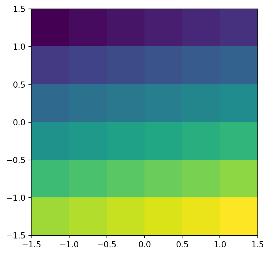

Figure 1.23: Plot of the `elev` raster, a minimal example of a continuous raster, created from scratch

The grain raster can be plotted the same way, as we are going to use the same transformation matrix for it as well (Figure fig-rasterio-plot-grain).

rasterio.plot.show(grain, transform=new_transform);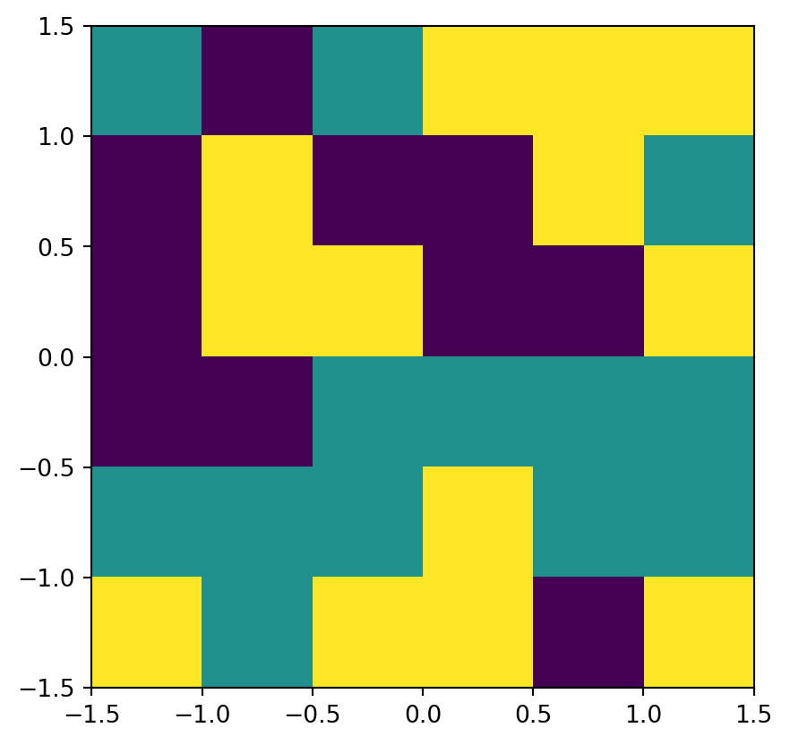

Figure 1.24: Plot of the `grain` raster, a minimal example of a categorical raster, created from scratch

At this point, we have two rasters, each composed of an array and related transformation matrix. We can work with the raster using rasterio by:

Passing the transformation matrix wherever actual raster pixel coordinates are important (such as in function rasterio.plot.show above)
Keeping in mind that any other layer we use in the analysis is in the same CRS

Finally, to export the raster for permanent storage, along with the spatial metadata, we need to go through the following steps:

Create a raster file connection (where we set the transform and the CRS, among other settings)
Write the array with raster values into the connection
Close the connection

Don’t worry if the code below is unclear; the concepts related to writing raster data to file will be explained in sec-data-output-raster. For now, for completeness, and also to use these rasters in subsequent chapters without having to re-create them from scratch, we just provide the code for exporting the elev and grain rasters into the output directory. In the case of elev, we do it as follows with the rasterio.open, .write, and .close functions and methods of the rasterio package.

new_dataset = rasterio.open(
    'output/elev.tif', 'w', 
    driver='GTiff',
    height=elev.shape[0],
    width=elev.shape[1],
    count=1,
    dtype=elev.dtype,
    crs=4326,
    transform=new_transform
)
new_dataset.write(elev, 1)
new_dataset.close()

Note that the CRS we (arbitrarily) set for the elev raster is WGS84, defined using crs=4326 according to the EPSG code.

Exporting the grain raster is done in the same way, with the only differences being the file name and the array we write into the connection.

new_dataset = rasterio.open(
    'output/grain.tif', 'w', 
    driver='GTiff',
    height=grain.shape[0],
    width=grain.shape[1],
    count=1,
    dtype=grain.dtype,
    crs=4326,
    transform=new_transform
)
new_dataset.write(grain, 1)
new_dataset.close()

As a result, the files elev.tif and grain.tif are written into the output directory. We are going to use these small raster files later on in the examples (for example, sec-raster-subsetting).

Note that the transform matrices and dimensions of elev and grain are identical. This means that the rasters are overlapping, and can be combined into one two-band raster, processed in raster algebra operations (sec-map-algebra), etc.

1.4 Coordinate Reference Systems

Vector and raster spatial data types share concepts intrinsic to spatial data. Perhaps the most fundamental of these is the Coordinate Reference System (CRS), which defines how the spatial elements of the data relate to the surface of the Earth (or other bodies). CRSs are either geographic or projected, as introduced at the beginning of this chapter (sec-vector-data). This section explains each type, laying the foundations for sec-reproj-geo-data, which provides a deep dive into setting, transforming, and querying CRSs.

1.4.1 Geographic coordinate systems

Geographic coordinate systems identify any location on the Earth’s surface using two values—longitude and latitude (see left panel of Figure fig-zion-crs). Longitude is a location in the East-West direction in angular distance from the Prime Meridian plane, while latitude is an angular distance North or South of the equatorial plane. Distances in geographic CRSs are therefore not measured in meters. This has important consequences, as demonstrated in sec-reproj-geo-data.

A spherical or ellipsoidal surface represents the surface of the Earth in geographic coordinate systems. Spherical models assume that the Earth is a perfect sphere of a given radius—they have the advantage of simplicity, but, at the same time, they are inaccurate: the Earth is not a sphere! Ellipsoidal models are defined by two parameters: the equatorial radius and the polar radius. These are suitable because the Earth is compressed: the equatorial radius is around 11.5 \(km\) longer than the polar radius. The Earth is not an ellipsoid either, but it is a better approximation than a sphere.

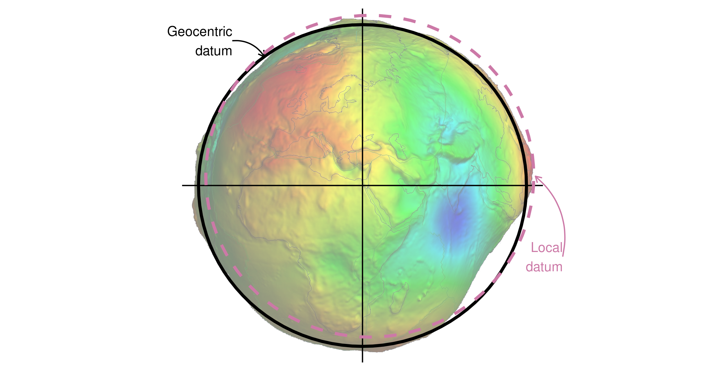
Ellipsoids are part of a broader component of CRSs: the datum. It contains information on what ellipsoid to use and the precise relationship between the Cartesian coordinates and location on the Earth’s surface. There are two types of datum—geocentric (such as WGS84) and local (such as NAD83). You can see examples of these two types of datums in Figure fig-geocentric-vs-local. Black lines represent a geocentric datum, whose center is located in the Earth’s center of gravity and is not optimized for a specific location. In a local datum, shown as a purple dashed line, the ellipsoidal surface is shifted to align with the surface at a particular location. These allow local variations on Earth’s surface, such as large mountain ranges, to be accounted for in a local CRS. This can be seen in Figure fig-geocentric-vs-local, where the local datum is fitted to the area of Philippines, but is misaligned with most of the rest of the planet’s surface. Both datums in Figure fig-geocentric-vs-local are put on top of a geoid—a model of global mean sea level.

Figure 1.25: Geocentric and local geodetic datums shown on top of a geoid (in false color and the vertical exaggeration by 10,000 scale factor). Image of the geoid is adapted from the work of (Ince et al. 2019).

1.4.2 Projected coordinate reference systems

All projected CRSs are based on a geographic CRS, described in the previous section, and rely on map projections to convert the three-dimensional surface of the Earth into Easting and Northing (x and y) values in a projected CRS. Projected CRSs are based on Cartesian coordinates on an implicitly flat surface (see right panel of Figure fig-zion-crs). They have an origin, x and y axes, and a linear unit of measurement such as meters.

This transition cannot be done without adding some deformations. Therefore, some properties of the Earth’s surface are distorted in this process, such as area, direction, distance, and shape. A projected coordinate system can preserve only one or two of those properties. Projections are often named based on a property they preserve: equal-area preserves area, azimuthal preserves direction, equidistant preserves distance, and conformal preserves local shape.

There are three main groups of projection types: conic, cylindrical, and planar (azimuthal). In a conic projection, the Earth’s surface is projected onto a cone along a single line of tangency or two lines of tangency. Distortions are minimized along the tangency lines and rise with the distance from those lines in this projection. Therefore, it is best suited for maps of mid-latitude areas. A cylindrical projection maps the surface onto a cylinder. This projection could also be created by touching the Earth’s surface along a single line of tangency or two lines of tangency. Cylindrical projections are used most often when mapping the entire world. A planar projection projects data onto a flat surface touching the globe at a point or along a line of tangency. It is typically used in mapping polar regions.

1.4.3 CRS in Python

Like most open-source geospatial software, the geopandas and rasterio packages use the PROJ software for CRS definition and calculations. The pyproj package is a low-level interface to PROJ. Using its functions, such as get_codes and from_epsg, we can examine the list of projections supported by PROJ.

import pyproj
epsg_codes = pyproj.get_codes('EPSG', 'CRS')  ## Supported EPSG codes
epsg_codes[:5]  ## Print first five supported EPSG codes

['10150', '10151', '10156', '10157', '10158']

pyproj.CRS.from_epsg(4326)  ## Printout of WGS84 CRS (EPSG:4326)

<Geographic 2D CRS: EPSG:4326>
Name: WGS 84
Axis Info [ellipsoidal]:
- Lat[north]: Geodetic latitude (degree)
- Lon[east]: Geodetic longitude (degree)
Area of Use:
- name: World.
- bounds: (-180.0, -90.0, 180.0, 90.0)
Datum: World Geodetic System 1984 ensemble
- Ellipsoid: WGS 84
- Prime Meridian: Greenwich

A quick summary of different projections, their types, properties, and suitability can be found at https://www.geo-projections.com/. We will expand on CRSs and explain how to project from one CRS to another in sec-reproj-geo-data. But, for now, it is sufficient to know:

That coordinate systems are a key component of geographic objects
Knowing which CRS your data is in, and whether it is in geographic (lon/lat) or projected (typically meters), is important and has consequences for how Python handles spatial and geometry operations
CRSs of geopandas (vector layer or geometry column) and rasterio (raster) objects can be queried with the .crs property

Here is a demonstration of the last bullet point, where we import a vector layer and figure out its CRS (in this case, a projected CRS, namely UTM Zone 12) using the .crs property.

zion = gpd.read_file('data/zion.gpkg')
zion.crs

<Bound CRS: PROJCS["UTM Zone 12, Northern Hemisphere",GEOGCS[" ...>
Name: UTM Zone 12, Northern Hemisphere
Axis Info [cartesian]:
- [east]: Easting (Meter)
- [north]: Northing (Meter)
Area of Use:
- undefined
Coordinate Operation:
- name: Transformation from GRS 1980(IUGG, 1980) to WGS84
- method: Position Vector transformation (geog2D domain)
Datum: unknown
- Ellipsoid: GRS80
- Prime Meridian: Greenwich
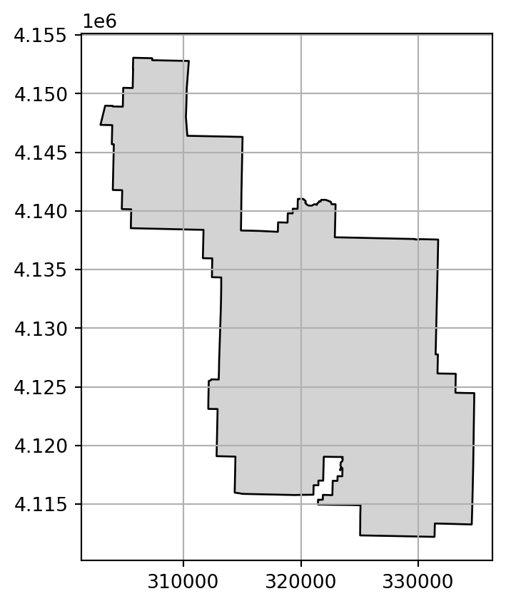
Source CRS: UTM Zone 12, Northern Hemisphere

We can also illustrate the difference between a geographic and a projected CRS by plotting the zion data in both CRSs (Figure fig-zion-crs). Note that we are using the .grid method of matplotlib to draw grid lines on top of the plot.

# WGS84
zion.to_crs(4326).plot(edgecolor='black', color='lightgrey').grid()
# NAD83 / UTM zone 12N
zion.plot(edgecolor='black', color='lightgrey').grid();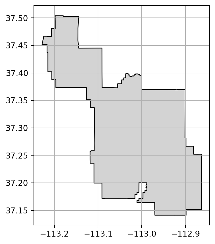

We are going to elaborate on reprojection from one CRS to another (.to_crs in the above code section) in sec-reproj-geo-data.

1.5 Units

An important feature of CRSs is that they contain information about spatial units. Clearly, it is vital to know whether a house’s measurements are in feet or meters, and the same applies to maps. It is a good cartographic practice to add a scale bar or some other distance indicator onto maps to demonstrate the relationship between distances on the page or screen and distances on the ground. Likewise, it is important for the user to be aware of the units in which the geometry coordinates are, to ensure that subsequent calculations are done in the right context.

Python spatial data structures in geopandas and rasterio do not natively support the concept of measurement units. The coordinates of a vector layer or a raster are plain numbers, referring to an arbitrary plane. For example, according to the .transform matrix of srtm.tif we can see that the raster resolution is 0.000833 and that its CRS is WGS84 (EPSG: 4326):

src.meta

{'driver': 'GTiff',
 'dtype': 'uint16',
 'nodata': 65535.0,
 'width': 465,
 'height': 457,
 'count': 1,
 'crs': CRS.from_epsg(4326),
 'transform': Affine(0.0008333333332777796, 0.0, -113.23958321278403,
        0.0, -0.0008333333332777843, 37.512916763165805)}

You may already know that the units of the WGS84 coordinate system (EPSG:4326) are decimal degrees. However, that information is not accounted for in any numeric calculation, meaning that operations such as buffers can be returned in units of degrees, which is not appropriate in most cases.

Consequently, you should always be aware of the CRS of your datasets and the units they use. Typically, these are decimal degrees, in a geographic CRS, or \(m\), in a projected CRS, although there are exceptions. Geometric calculations such as length, area, or distance, return plain numbers in the same units of the CRS (such as \(m\) or \(m^2\)). It is up to the user to determine which units the result is given in, and treat the result accordingly. For example, if the area output was in \(m^2\) and we need the result in \(km^2\), then we need to divide the result by \(1000^2\).

Bossche, Joris Van den, Kelsey Jordahl, Martin Fleischmann, James McBride, Jacob Wasserman, Matt Richards, Adrian Garcia Badaracco, et al. 2023. “Geopandas/Geopandas: V0.14.0.” Zenodo. https://doi.org/10.5281/zenodo.8348034.

Gillies, Sean et al. 2007--. “Shapely: Manipulation and Analysis of Geometric Objects.” toblerity.org. https://github.com/Toblerity/Shapely.

Harris, Charles R., K. Jarrod Millman, Stéfan J. van der Walt, Ralf Gommers, Pauli Virtanen, David Cournapeau, Eric Wieser, et al. 2020. “Array Programming with NumPy.” Nature 585 (7825): 357–62. https://doi.org/10.1038/s41586-020-2649-2.

Ince, E. S., F. Barthelmes, S. Reißland, K. Elger, C. Förste, F. Flechtner, and H. Schuh. 2019. “ICGEM – 15 Years of Successful Collection and Distribution of Global Gravitational Models, Associated Services, and Future Plans.” Earth System Science Data 11 (2): 647–74. https://doi.org/gg5tzm.

McKinney, Wes. 2010. “Data Structures for Statistical Computing in Python.” In Proceedings of the 9th Python in Science Conference, edited by Stéfan van der Walt and Jarrod Millman, 56–61. https://doi.org/ 10.25080/Majora-92bf1922-00a .

Pebesma, Edzer, and Roger Bivand. 2022. Spatial Data Science with Applications in R. https://r-spatial.org/book.

Tennekes, Martijn, and Jakub Nowosad. 2022. Elegant and Informative Maps with Tmap.

https://r-spatial.github.io/sf/articles/sf1.html#simple-feature-geometry-types ↩︎