7 Geographic data I/O

Prerequisites

This chapter requires importing the following packages:

import urllib.request
import zipfile
import numpy as np
import matplotlib.pyplot as plt
import pandas as pd
import shapely
import pyogrio
import geopandas as gpd
import rasterio
import rasterio.plot
import cartopy
import osmnx as ox

It also relies on the following data files:

nz = gpd.read_file('data/nz.gpkg')
nz_elev = rasterio.open('data/nz_elev.tif')

7.1 Introduction

This chapter is about reading and writing geographic data. Geographic data input is essential for geocomputation: real-world applications are impossible without data. Data output is also vital, enabling others to use valuable new or improved datasets resulting from your work. Taken together, these processes of input/output can be referred to as data I/O.

Geographic data I/O is often done with few lines of code at the beginning and end of projects. It is often overlooked as a simple one-step process. However, mistakes made at the outset of projects (e.g., using an out-of-date or in some way faulty dataset) can lead to large problems later down the line, so it is worth putting considerable time into identifying which datasets are available, where they can be found and how to retrieve them. These topics are covered in Section 7.2, which describes several geoportals, which collectively contain many terabytes of data, and how to use them. To further ease data access, a number of packages for downloading geographic data have been developed, as demonstrated in Section 7.3.

There are many geographic file formats, each of which has pros and cons, described in Section 7.4. The process of reading and writing files efficiently is covered in Section 7.5 and Section 7.6, respectively.

7.2 Retrieving open data

A vast and ever-increasing amount of geographic data is available on the internet, much of which is free to access and use (with appropriate credit given to its providers)¹. In some ways there is now too much data, in the sense that there are often multiple places to access the same dataset. Some datasets are of poor quality. In this context, it is vital to know where to look, so the first section covers some of the most important sources. Various ‘geoportals’ (web services providing geospatial datasets, such as Data.gov²) are a good place to start, providing a wide range of data but often only for specific locations (as illustrated in the updated Wikipedia page³ on the topic).

Some global geoportals overcome this issue. The GEOSS portal⁴ and the Copernicus Data Space Ecosystem⁵, for example, contain many raster datasets with global coverage. A wealth of vector datasets can be accessed from the SEDAC⁶ portal run by the National Aeronautics and Space Administration (NASA) and the European Union’s INSPIRE geoportal⁷, with global and regional coverage.

Most geoportals provide a graphical interface allowing datasets to be queried based on characteristics such as spatial and temporal extent, the United States Geological Survey’s EarthExplorer⁸ and NASA’s EarthData Search⁹ being prime examples. Exploring datasets interactively on a browser is an effective way of understanding available layers. From reproducibility and efficiency perspectives, downloading data is, however, best done with code. Downloads can be initiated from the command line using a variety of techniques, primarily via URLs and APIs (see the Sentinel API¹⁰, for example).

Files hosted on static URLs can be downloaded with the following method, as illustrated in the code chunk below which accesses the Natural Earth Data¹¹ website to download the world airports layer zip file and to extract the contained ESRI Shapefile. Note that the download code is complicated by the fact that the server checks the User-agent header of the request, basically to make sure that the download takes place through a browser. To overcome this, we add a header corresponding to a request coming from a browser (such as Firefox) in our code.

# Set URL+filename
url = 'https://naciscdn.org/naturalearth/10m/cultural/ne_10m_airports.zip'
filename = 'output/ne_10m_airports.zip'
# Download
urllib.request.urlretrieve(url, filename)
# Extract
f = zipfile.ZipFile(filename, 'r')
f.extractall('output')
f.close()

The ESRI Shapefile that has been created in the output directory can then be imported and plotted (Figure 7.1) as follows using geopandas.

ne = gpd.read_file(filename.replace('.zip', '.shp'))
ne.plot();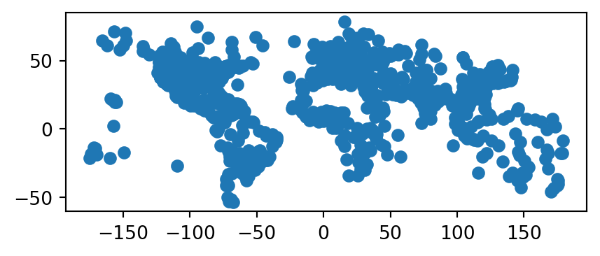

Figure 7.1: World airports layer, downloaded from the Natural Earth Data website using Python

7.3 Geographic data packages

Several Python packages have been developed for accessing geographic data, two of which are demonstrated below. These provide interfaces to one or more spatial libraries or geoportals and aim to make data access even quicker from the command line.

Administrative borders are often useful in spatial analysis. These can be accessed with the cartopy.io.shapereader.natural_earth function from the cartopy package (Met Office 2010-2015). For example, the following code loads the 'admin_2_counties' dataset of US counties into a GeoDataFrame.

filename = cartopy.io.shapereader.natural_earth(
    resolution='10m',
    category='cultural',
    name='admin_2_counties'
)
counties = gpd.read_file(filename)
counties

/usr/local/lib/python3.11/site-packages/cartopy/io/__init__.py:241: DownloadWarning: Downloading: https://naturalearth.s3.amazonaws.com/10m_cultural/ne_10m_admin_2_counties.zip
  warnings.warn(f'Downloading: {url}', DownloadWarning)

	FEATURECLA	SCALERANK	...	NAME_ZHT	geometry
0	Admin-2 scale rank	0	...	霍特科姆縣	MULTIPOLYGON (((-122.75302 48.9...
1	Admin-2 scale rank	0	...	奧卡諾根縣	POLYGON ((-120.85196 48.99251, ...
2	Admin-2 scale rank	0	...	費里縣	POLYGON ((-118.83688 48.99251, ...
...	...	...	...	...	...
3221	Admin-2 scale rank	0	...	維拉爾巴	POLYGON ((-66.44407 18.17665, -...
3222	Admin-2 scale rank	0	...	大薩瓦納	POLYGON ((-66.88464 18.02481, -...
3223	Admin-2 scale rank	0	...	馬里考	POLYGON ((-66.89856 18.1879, -6...

3224 rows × 62 columns

The resulting layer counties is shown in Figure 7.2.

counties.plot();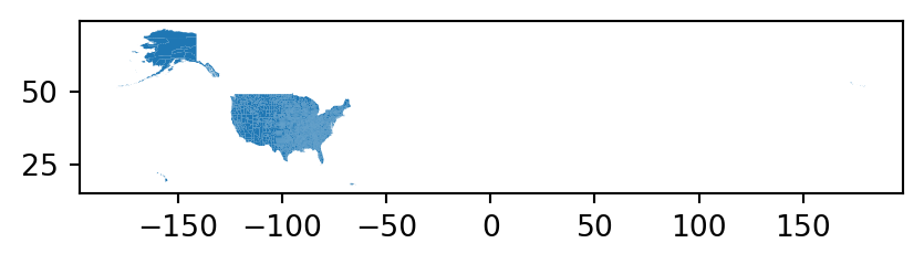

Figure 7.2: US counties, downloaded from the Natural Earth Data website using package **cartopy**

Note that Figure 7.2 x-axis spans the entire range of longitudes, between -180 and 180, since the Aleutian Islands county (which is small and difficult to see on the map) crosses the International Date Line.

Other layers can from NaturalEarth be accessed the same way. You need to specify the resolution, category, and name of the requested dataset in Natural Earth Data, then run the cartopy.io.shapereader.natural_earth, which downloads the file(s) and returns the path, and read the file into the Python environment, e.g., using gpd.read_file. This is an alternative approach to ‘directly’ downloading files as shown earlier (Section 7.2).

The second example uses the osmnx package (Boeing 2017) to find parks from the OpenStreetMap (OSM) database. As illustrated in the code chunk below, OpenStreetMap data can be obtained using the ox.features.features_from_place function. The first argument is a string which is geocoded to a polygon (the ox.features.features_from_bbox and ox.features.features_from_polygon can also be used to query a custom area of interest). The second argument specifies the OSM tag(s)¹², selecting which OSM elements we’re interested in (parks, in this case), represented by key-value pairs.

parks = ox.features.features_from_place(
    query='leeds uk', 
    tags={'leisure': 'park'}
)

The result is a GeoDataFrame with the parks in Leeds. Now, we can plot the geometries with the name property in the tooltips using explore (Figure 7.3).

parks[['name', 'geometry']].explore()

Make this Notebook Trusted to load map: File -> Trust Notebook

Figure 7.3: Parks in Leeds, based on OpenStreetMap data, downloaded using package osmnx

It should be noted that the osmnx package downloads OSM data from the Overpass API¹³, which is rate limited and therefore unsuitable for queries covering very large areas. To overcome this limitation, you can download OSM data extracts, such as in Shapefile format from Geofabrik¹⁴, and then load them from the file into the Python environment.

OpenStreetMap is a vast global database of crowd-sourced data, is growing daily, and has a wider ecosystem of tools enabling easy access to the data, from the Overpass turbo¹⁵ web service for rapid development and testing of OSM queries to osm2pgsql for importing the data into a PostGIS database. Although the quality of datasets derived from OSM varies, the data source and wider OSM ecosystems have many advantages: they provide datasets that are available globally, free of charge, and constantly improving thanks to an army of volunteers. Using OSM encourages ‘citizen science’ and contributions back to the digital commons (you can start editing data representing a part of the world you know well at https://www.openstreetmap.org/).

One way to obtain spatial information is to perform geocoding—transform a description of a location, usually an address, into a set of coordinates. This is typically done by sending a query to an online service and getting the location as a result. Many such services exist that differ in the used method of geocoding, usage limitations, costs, or API key requirements. Nominatim¹⁶ is a well-known free service, based on OpenStreetMap data, and there are many other free and commercial geocoding services.

geopandas provides the gpd.tools.geocode function, which can geocode addresses to a GeoDataFrame. Internally it uses the geopy package, supporting several providers through the provider parameter (use geopy.geocoders.SERVICE_TO_GEOCODER to see possible options). The example below searches for John Snow blue plaque¹⁷ coordinates located on a building in the Soho district of London. The result is a GeoDataFrame with the address we passed to gpd.tools.geocode, and the detected point location.

result = gpd.tools.geocode('54 Frith St, London W1D 4SJ, UK', timeout=10)
result

	geometry	address
0	POINT (-0.13178 51.51377)	54, Frith Street, W1D 3JD, Frit...

Importantly, (1) we can pass a list of multiple addresses instead of just one, resulting in a GeoDataFrame with corresponding multiple rows, and (2) ‘No Results’ responses are represented by POINT EMPTY geometries, as shown in the following example.

result = gpd.tools.geocode(
    ['54 Frith St, London W1D 4SJ, UK', 'abcdefghijklmnopqrstuvwxyz'], 
    timeout=10
)
result

	geometry	address
0	POINT (-0.13178 51.51377)	54, Frith Street, W1D 3JD, Frit...
1	POINT EMPTY	None

The result is visualized in Figure 7.4 using the .explore function. We are using the marker_kwds parameter of .explore to make the marker larger (see Section 8.3.2).

result.iloc[[0]].explore(color='red', marker_kwds={'radius':20})

Make this Notebook Trusted to load map: File -> Trust Notebook

Figure 7.4: Specific address in London, geocoded into a GeoDataFrame

7.4 File formats

Geographic datasets are usually stored as files or in spatial databases. File formats usually can either store vector or raster data, while spatial databases such as PostGIS can store both. The large variety of file formats may seem bewildering, but there has been much consolidation and standardization since the beginnings of GIS software in the 1960s when the first widely distributed program SYMAP for spatial analysis was created at Harvard University (Coppock and Rhind 1991).

GDAL (which originally was pronounced as ‘goo-dal’, with the double ‘o’ making a reference to object-orientation), the Geospatial Data Abstraction Library, has resolved many issues associated with incompatibility between geographic file formats since its release in 2000. GDAL provides a unified and high-performance interface for reading and writing of many raster and vector data formats. Many open and proprietary GIS programs, including GRASS, ArcGIS and QGIS, use GDAL behind their GUIs for doing the legwork of ingesting and spitting out geographic data in appropriate formats. Most Python packages for working with spatial data, including geopandas and rasterio used in this book, also rely on GDAL for importing and exporting spatial data files.

GDAL provides access to more than 200 vector and raster data formats. Table 7.1 presents some basic information about selected and often-used spatial file formats.

Table 7.1: Commonly used spatial data file formats

Name	Extension	Info	Type	Model
ESRI Shapefile	`.shp` (the main file)	Popular format consisting of at least three files. No support for: files > 2GB; mixed types; names > 10 chars; cols > 255.	Vector	Partially open
GeoJSON	`.geojson`	Extends the JSON exchange format by including a subset of the simple feature representation; mostly used for storing coordinates in longitude and latitude; it is extended by the TopoJSON format.	Vector	Open
KML	`.kml`	XML-based format for spatial visualization, developed for use with Google Earth. Zipped KML file forms the KMZ format.	Vector	Open
GPX	`.gpx`	XML schema created for exchange of GPS data.	Vector	Open
FlatGeobuf	`.fgb`	Single file format allowing for quick reading and writing of vector data. Has streaming capabilities.	Vector	Open
GeoTIFF	`.tif/.tiff`	Popular raster format. A TIFF file containing additional spatial metadata.	Raster	Open
Arc ASCII	`.asc`	Text format where the first six lines represent the raster header, followed by the raster cell values arranged in rows and columns.	Raster	Open
SQLite/SpatiaLite	`.sqlite`	Standalone relational database, SpatiaLite is the spatial extension of SQLite.	Vector and raster	Open
ESRI FileGDB	`.gdb`	Spatial and nonspatial objects created by ArcGIS. Allows: multiple feature classes; topology. Limited support from GDAL.	Vector and raster	Proprietary
GeoPackage	`.gpkg`	Lightweight database container based on SQLite allowing an easy and platform-independent exchange of geodata.	Vector and (very limited) raster	Open

An important development ensuring the standardization and open-sourcing of file formats was the founding of the Open Geospatial Consortium (OGC) in 1994. Beyond defining the Simple Features data model (see Section 1.2.4), the OGC also coordinates the development of open standards, for example as used in file formats such as KML and GeoPackage. Open file formats of the kind endorsed by the OGC have several advantages over proprietary formats: the standards are published, ensure transparency and open up the possibility for users to further develop and adjust the file formats to their specific needs.

ESRI Shapefile is the most popular vector data exchange format; however, it is not a fully open format (though its specification is open). It was developed in the early 1990s and, from a modern standpoint, has a number of limitations. First of all, it is a multi-file format, which consists of at least three files. It also only supports 255 columns, its column names are restricted to ten characters and the file size limit is 2 GB. Furthermore, ESRI Shapefile does not support all possible geometry types, for example, it is unable to distinguish between a polygon and a multipolygon. Despite these limitations, a viable alternative had been missing for a long time. In 2014, GeoPackage emerged, and seems to be a more than suitable replacement candidate for ESRI Shapefile. GeoPackage is a format for exchanging geospatial information and an OGC standard. This standard describes the rules on how to store geospatial information in a tiny SQLite container. Hence, GeoPackage is a lightweight spatial database container, which allows the storage of vector and raster data but also of non-spatial data and extensions. Aside from GeoPackage, there are other geospatial data exchange formats worth checking out (Table 7.1).

The GeoTIFF format seems to be the most prominent raster data format. It allows spatial information, such as the CRS definition and the transformation matrix (see Section 1.3.1), to be embedded within a TIFF file. Similar to ESRI Shapefile, this format was firstly developed in the 1990s, but as an open format. Additionally, GeoTIFF is still being expanded and improved. One of the most significant recent additions to the GeoTIFF format is its variant called COG (Cloud Optimized GeoTIFF). Raster objects saved as COGs can be hosted on HTTP servers, so other people can read only parts of the file without downloading the whole file (Section 7.5.2).

There is also a plethora of other spatial data formats that we do not explain in detail or mention in Table 7.1 due to the book limits. If you need to use other formats, we encourage you to read the GDAL documentation about vector and raster drivers. Additionally, some spatial data formats can store other data models (types) than vector or raster. Two examples are LAS and LAZ formats for storing lidar point clouds, and NetCDF and HDF for storing multidimensional arrays.

Finally, spatial data are also often stored using tabular (non-spatial) text formats, including CSV files or Excel spreadsheets. This can be convenient to share spatial (point) datasets with people who, or software that, struggle with spatial data formats. If necessary, the table can be converted to a point layer (see examples in Section 1.2.6 and Section 3.2.3).

7.5 Data input (I)

Executing commands such as gpd.read_file (the main function we use for loading vector data) or rasterio.open+.read (the main group of functions used for loading raster data) silently sets off a chain of events that reads data from files. Moreover, there are many Python packages containing a wide range of geographic data or providing simple access to different data sources. All of them load the data into the Python environment or, more precisely, assign objects to your workspace, stored in RAM and accessible within the Python session. The latter is the most straightforward approach, suitable when RAM is not a limiting factor. For large vector layers and rasters, partial reading may be required. For vector layers, we will demonstrate how to read subsets of vector layers, filtered by attributes or by location (Section 7.5.1). For rasters, we already showed earlier in the book how the user can choose which specific bands to read (Section 1.3.1), or read resampled data to a lower resolution (Section 4.3.2). In this section, we also show how to read specific rectangular extents (‘windows’) from a raster file (Section 7.5.2).

7.5.1 Vector data

Spatial vector data comes in a wide variety of file formats. Most popular representations such as .shp, .geojson, and .gpkg files can be imported and exported with geopandas function gpd.read_file and method .to_file (covered in Section 7.6), respectively.

geopandas uses GDAL to read and write data, via pyogrio since geopandas version 1.0.0 (previously via fiona). After pyogrio is imported, pyogrio.list_drivers can be used to list drivers available to GDAL, including whether they can read ('r'), append ('a'), or write ('w') data, or all three.

pyogrio.list_drivers()

{'PCIDSK': 'rw',
 'PDS4': 'rw',
 ...
 'AVCE00': 'r',
 'HTTP': 'r'}

The first argument of the geopandas versatile data import function gpd.read_file is filename, which is typically a string, but can also be a file connection. The content of a string could vary between different drivers. In most cases, as with the ESRI Shapefile (.shp) or the GeoPackage format (.gpkg), the filename argument would be a path or a URL to an actual file, such as geodata.gpkg. The driver is automatically selected based on the file extension, as demonstrated for a .gpkg file below.

world = gpd.read_file('data/world.gpkg')

For some drivers, such as a File Geodatabase (OpenFileGDB), filename could be provided as a folder name. GeoJSON, a plain text format, on the other hand, can be read from a .geojson file, but also from a string.

gpd.read_file('{"type":"Point","coordinates":[34.838848,31.296301]}')

	geometry
0	POINT (34.83885 31.2963)

Some vector formats, such as GeoPackage, can store multiple data layers. By default, gpd.read_file reads the first layer of the file specified in filename. However, using the layer argument you can specify any other layer. To list the available layers, we can use function gpd.list_layers (or pyogrio.list_layers).

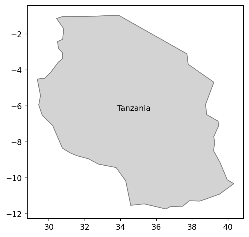
The gpd.read_file function also allows for reading just parts of the file into RAM with two possible mechanisms. The first one is related to the where argument, which allows specifying what part of the data to read using an SQL WHERE expression. An example below extracts data for Tanzania only from the world.gpkg file (Figure 7.5 (a)). It is done by specifying that we want to get all rows for which name_long equals to 'Tanzania'.

tanzania = gpd.read_file('data/world.gpkg', where='name_long="Tanzania"')
tanzania

	iso_a2	name_long	...	gdpPercap	geometry
0	TZ	Tanzania	...	2402.099404	MULTIPOLYGON (((33.90371 -0.95,...

1 rows × 11 columns

If you do not know the names of the available columns, a good approach is to read the layer metadata using pyogrio.read_info. The resulting object contains, among other properties, the column names (fields) and data types (dtypes):

info = pyogrio.read_info('data/world.gpkg')
info['fields']

array(['iso_a2', 'name_long', 'continent', 'region_un', 'subregion',
       'type', 'area_km2', 'pop', 'lifeExp', 'gdpPercap'], dtype=object)

info['dtypes']

array(['object', 'object', 'object', 'object', 'object', 'object',
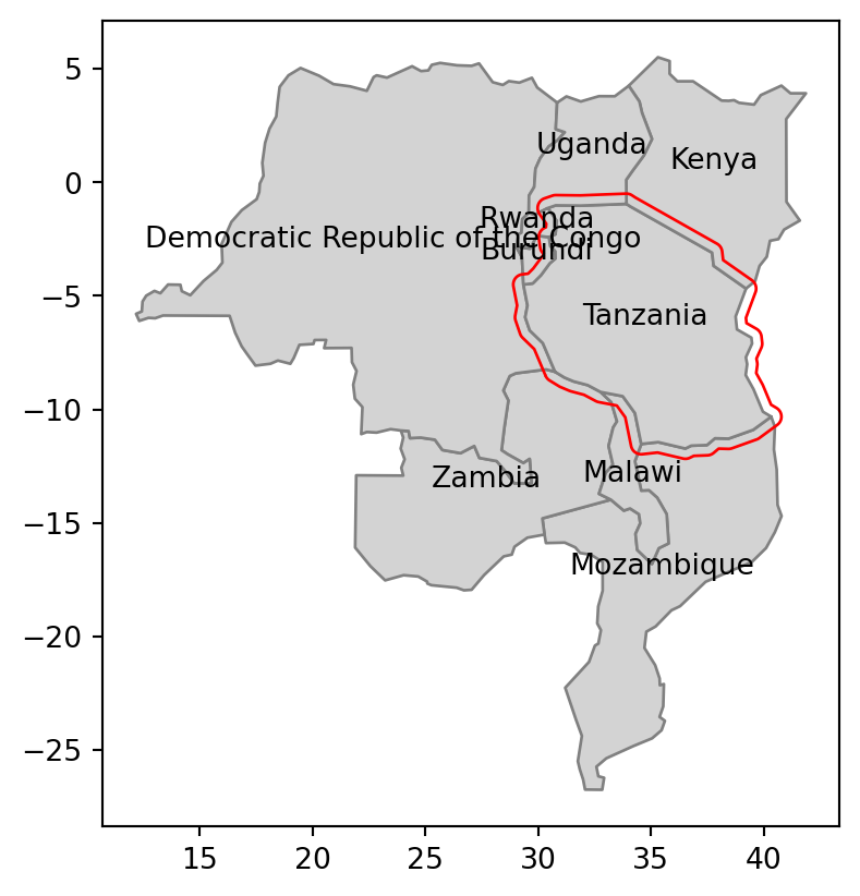
       'float64', 'float64', 'float64', 'float64'], dtype=object)

The second mechanism uses the mask argument to filter data based on intersection with an existing geometry. This argument expects a geometry (GeoDataFrame, GeoSeries, or shapely geometry) representing the area where we want to extract the data. Let’s try it using a small example—we want to read polygons from our file that intersect with the buffer of 50,000 \(m\) of Tanzania’s borders. To do it, we need to transform the geometry to a projected CRS (such as EPSG:32736), prepare our ‘filter’ by creating the buffer (Section 4.2.3), and transform back to the original CRS to be used as a mask (Figure 7.5 (a)).

tanzania_buf = tanzania.to_crs(32736).buffer(50000).to_crs(4326)

Now, we can pass the ‘filter’ geometry tanzania_buf to the mask argument of gpd.read_file.

tanzania_neigh = gpd.read_file('data/world.gpkg', mask=tanzania_buf)

Our result, shown in Figure 7.5 (b), contains Tanzania and every country intersecting with its 50,000 \(m\) buffer. Note that the last two expressions are used to add text labels with the name_long of each country, placed at the country centroid.

# Using 'where'
fig, ax = plt.subplots()
tanzania.plot(ax=ax, color='lightgrey', edgecolor='grey')
tanzania.apply(
    lambda x: ax.annotate(text=x['name_long'], 
    xy=x.geometry.centroid.coords[0], ha='center'), axis=1
);
# Using 'mask'
fig, ax = plt.subplots()
tanzania_neigh.plot(ax=ax, color='lightgrey', edgecolor='grey')
tanzania_buf.plot(ax=ax, color='none', edgecolor='red')
tanzania_neigh.apply(
    lambda x: ax.annotate(text=x['name_long'],
    xy=x.geometry.centroid.coords[0], ha='center'), axis=1
);

(a) Using a `where` query (matching `'Tanzania'`)

A different, gpd.read_postgis, function can be used to read a vector layer from a PostGIS database.

Often we need to read CSV files (or other tabular formats) which have x and y coordinate columns, and turn them into a GeoDataFrame with point geometries. To do that, we can import the file using pandas (e.g., using pd.read_csv or pd.read_excel), then go from DataFrame to GeoDataFrame using the gpd.points_from_xy function, as shown earlier in the book (See Section 1.2.6 and Section 3.2.3). For example, the table cycle_hire_xy.csv, where the coordinates are stored in the X and Y columns in EPSG:4326, can be imported, converted to a GeoDataFrame, and plotted, as follows (Figure 7.6).

cycle_hire = pd.read_csv('data/cycle_hire_xy.csv')
geom = gpd.points_from_xy(cycle_hire['X'], cycle_hire['Y'], crs=4326)
geom = gpd.GeoSeries(geom)
cycle_hire_xy = gpd.GeoDataFrame(data=cycle_hire, geometry=geom)
cycle_hire_xy.plot();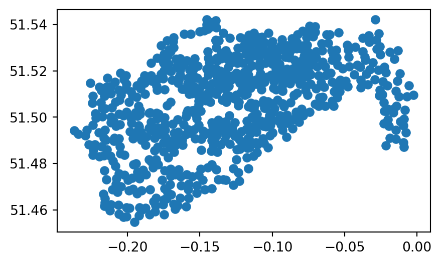

Figure 7.6: The `cycle_hire_xy.csv` table transformed to a point layer

Instead of columns describing ‘XY’ coordinates, a single column can also contain the geometry information, not necessarily points but possibly any other geometry type. Well-known text (WKT), well-known binary (WKB), and GeoJSON are examples of formats used to encode geometry in such a column. For instance, the world_wkt.csv file has a column named 'WKT', representing polygons of the world’s countries (in WKT format). When importing the CSV file into a DataFrame, the 'WKT' column is interpreted just like any other string column.

world_wkt = pd.read_csv('data/world_wkt.csv')
world_wkt

	WKT	iso_a2	...	lifeExp	gdpPercap
0	MULTIPOLYGON (((180.0 -16.06713...	FJ	...	69.960000	8222.253784
1	MULTIPOLYGON (((33.903711197104...	TZ	...	64.163000	2402.099404
2	MULTIPOLYGON (((-8.665589565454...	EH	...	NaN	NaN
...	...	...	...	...	...
174	MULTIPOLYGON (((20.590246546680...	XK	...	71.097561	8698.291559
175	MULTIPOLYGON (((-61.68 10.76,-6...	TT	...	70.426000	31181.821196
176	MULTIPOLYGON (((30.833852421715...	SS	...	55.817000	1935.879400

177 rows × 11 columns

To convert it to a GeoDataFrame, we can apply the gpd.GeoSeries.from_wkt function (which is analogous to shapely’s shapely.from_wkt, see Section 1.2.5) on the WKT strings, to convert the series of WKT strings into a GeoSeries with the geometries.

world_wkt['geometry'] = gpd.GeoSeries.from_wkt(world_wkt['WKT'])
world_wkt = gpd.GeoDataFrame(world_wkt)
world_wkt

	WKT	iso_a2	...	gdpPercap	geometry
0	MULTIPOLYGON (((180.0 -16.06713...	FJ	...	8222.253784	MULTIPOLYGON (((180 -16.06713, ...
1	MULTIPOLYGON (((33.903711197104...	TZ	...	2402.099404	MULTIPOLYGON (((33.90371 -0.95,...
2	MULTIPOLYGON (((-8.665589565454...	EH	...	NaN	MULTIPOLYGON (((-8.66559 27.656...
...	...	...	...	...	...
174	MULTIPOLYGON (((20.590246546680...	XK	...	8698.291559	MULTIPOLYGON (((20.59025 41.855...
175	MULTIPOLYGON (((-61.68 10.76,-6...	TT	...	31181.821196	MULTIPOLYGON (((-61.68 10.76, -...
176	MULTIPOLYGON (((30.833852421715...	SS	...	1935.879400	MULTIPOLYGON (((30.83385 3.5091...

177 rows × 12 columns

The resulting layer is shown in Figure 7.7.

world_wkt.plot();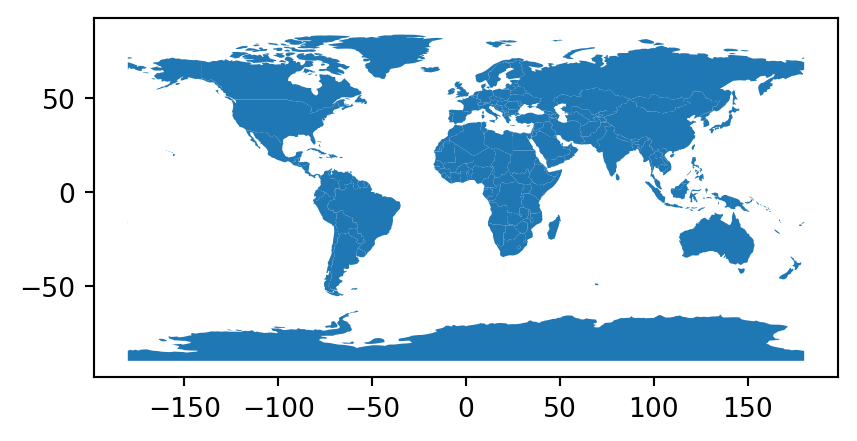

Figure 7.7: The `world_wkt.csv` table transformed to a polygon layer

As a final example, we will show how geopandas also reads KML files. A KML file stores geographic information in XML format—a data format for the creation of web pages and the transfer of data in an application-independent way (Nolan and Lang 2014). Here, we access a KML file from the web.

The sample KML file KML_Samples.kml contains more than one layer.

u = 'https://developers.google.com/kml/documentation/KML_Samples.kml'
gpd.list_layers(u)

	name	geometry_type
0	Placemarks	Point Z
1	Highlighted Icon	Point Z
2	Paths	LineString Z
3	Google Campus	Polygon Z
4	Extruded Polygon	Polygon Z
5	Absolute and Relative	Polygon Z

We can choose, for instance, the first layer 'Placemarks' and read it, using gpd.read_file with an additional layer argument.

placemarks = gpd.read_file(u, layer='Placemarks')
placemarks

	Name	Description	geometry
0	Simple placemark	Attached to the ground. Intelli...	POINT Z (-122.0822 37.42229 0)
1	Floating placemark	Floats a defined distance above...	POINT Z (-122.08408 37.422 50)
2	Extruded placemark	Tethered to the ground by a cus...	POINT Z (-122.08577 37.42157 50)

7.5.2 Raster data

Similar to vector data, raster data comes in many file formats, some of which support multilayer files. rasterio.open is used to create a file connection to a raster file, which can be subsequently used to read the metadata and/or the values, as shown previously (Section 1.3.1).

src = rasterio.open('data/srtm.tif')
src

<open DatasetReader name='data/srtm.tif' mode='r'>

All of the previous examples, like the one above, read spatial information from files stored on your hard drive. However, GDAL also allows reading data directly from online resources, such as HTTP/HTTPS/FTP web resources. Let’s try it by connecting to the global monthly snow probability at 500 \(m\) resolution for the period 2000-2012 (Hengl 2021). Snow probability for December is stored as a Cloud Optimized GeoTIFF (COG) file (see Section 7.4) and can be accessed by its HTTPS URI.

url = 'https://zenodo.org/record/5774954/files/'
url += 'clm_snow.prob_esacci.dec_p.90_500m_s0..0cm_2000..2012_v2.0.tif'
src = rasterio.open(url)
src

<open DatasetReader name='https://zenodo.org/record/5774954/files/clm_snow.prob_esacci.dec_p.90_500m_s0..0cm_2000..2012_v2.0.tif' mode='r'>

In the example above rasterio.open creates a connection to the file without obtaining any values, as we did for the local srtm.tif file. The values can be read into an ndarray using the .read method of the file connection (Section 1.3.1). Using parameters of .read allows us to just read a small portion of the data, without downloading the entire file. This is very useful when working with large datasets hosted online from resource-constrained computing environments such as laptops.

For example, we can read a specified rectangular extent of the raster. With rasterio, this is done using the so-called windowed reading capabilities. Note that, with windowed reading, we import just a subset of the raster extent into an ndarray covering any partial extent. Windowed reading is therefore memory- (and, in this case, bandwidth-) efficient, since it avoids reading the entire raster into memory. It can also be considered an alternative pathway to cropping (Section 5.2).

To read a raster window, let’s first define the bounding box coordinates. For example, here we use a \(10 \times 10\) degrees extent coinciding with Reykjavik.

xmin=-30
xmax=-20
ymin=60
ymax=70

Using the extent coordinates along with the raster transformation matrix, we create a window object, using the rasterio.windows.from_bounds function. This function basically ‘translates’ the extent from coordinates, to row/column ranges.

w = rasterio.windows.from_bounds(
    left=xmin, 
    bottom=ymin,
    right=xmax,
    top=ymax, 
    transform=src.transform
)
w

Window(col_off=35999.99999999998, row_off=4168.799999999996, width=2399.9999999999927, height=2400.0)

Now we can read the partial array, according to the specified window w, by passing it to the .read method.

r = src.read(1, window=w)
r

array([[100, 100, 100, ..., 255, 255, 255],
       [100, 100, 100, ..., 255, 255, 255],
       [100, 100, 100, ..., 255, 255, 255],
       ...,
       [255, 255, 255, ..., 255, 255, 255],
       [255, 255, 255, ..., 255, 255, 255],
       [255, 255, 255, ..., 255, 255, 255]], dtype=uint8)

Note that the transformation matrix of the window is not the same as that of the original raster (unless it incidentally starts from the top-left corner)! Therefore, we must re-create the transformation matrix, with the modified origin (xmin,ymax), yet the same resolution, as follows.

w_transform = rasterio.transform.from_origin(
    west=xmin, 
    north=ymax, 
    xsize=src.transform[0],
    ysize=abs(src.transform[4])
)
w_transform

Affine(0.00416666666666667, 0.0, -30.0,
       0.0, -0.00416666666666667, 70.0)

The array r along with the updated transformation matrix w_transform comprise the partial window, which we can keep working with just like with any other raster, as shown in previous chapters. Figure 7.8 shows the result, along with the location of Reykjavik.

fig, ax = plt.subplots()
rasterio.plot.show(r, transform=w_transform, ax=ax)
gpd.GeoSeries(shapely.Point(-21.94, 64.15)).plot(ax=ax, color='red');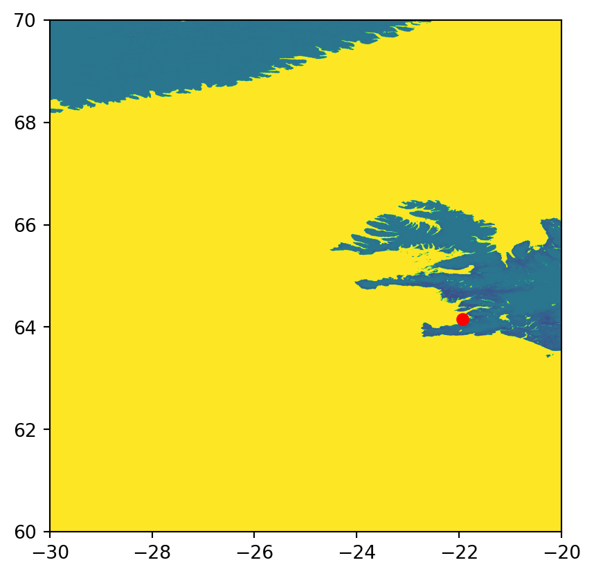

Figure 7.8: Raster window read from a remote Cloud Optimized GeoTIFF (COG) file source

Another option is to extract raster values at particular points, directly from the file connection, using the .sample method (see Section 3.3.1). For example, we can get the snow probability for December in Reykjavik (70%) by specifying its coordinates and applying .sample.

coords = (-21.94, 64.15)
values = src.sample([coords])
list(values)

[array([70], dtype=uint8)]

The example above efficiently extracts and downloads a single value instead of the entire GeoTIFF file, saving valuable resources.

Note that URIs can also identify vector datasets, enabling you to import datasets from online storage with geopandas, including datasets within ZIP archives hosted on the web.

gpd.read_file("zip+https://github.com/Toblerity/Fiona/files/11151652/coutwildrnp.zip")

	PERIMETER	FEATURE2	...	STATE	geometry
0	1.221070	None	...	UT	POLYGON ((-111.73528 41.99509, ...
1	0.755827	None	...	UT	POLYGON ((-112.00385 41.5527, -...
2	1.708510	None	...	CO	POLYGON ((-106.79289 40.98353, ...
...	...	...	...	...	...
64	0.263251	None	...	CO	POLYGON ((-108.35329 37.26869, ...
65	0.119581	None	...	CO	POLYGON ((-108.44212 37.29754, ...
66	0.120627	None	...	CO	POLYGON ((-108.5527 37.28285, -...

67 rows × 11 columns

7.6 Data output (O)

Writing geographic data allows you to convert from one format to another and to save newly created objects for permanent storage. Depending on the data type (vector or raster), object class (e.g., GeoDataFrame), and type and amount of stored information (e.g., object size, range of values), it is important to know how to store spatial files in the most efficient way. The next two subsections will demonstrate how to do this.

7.6.1 Vector data

The counterpart of gpd.read_file is the .to_file method that a GeoDataFrame has. It allows you to write GeoDataFrame objects to a wide range of geographic vector file formats, including the most common ones, such as .geojson, .shp and .gpkg. Based on the file name, .to_file decides automatically which driver to use. The speed of the writing process depends also on the driver.

For example, to export the world layer to a GeoPackage file, we can use .to_file and specify the output file name.

world.to_file('output/world.gpkg')

Note, that if you try to write to the same data source again, the function will overwrite the file.

world.to_file('output/world.gpkg')

Instead of overwriting the file, we could add new rows to the file with mode='a' (‘append’ mode, as opposed to the default mode='w' for the ‘write’ mode). Appending is supported by several spatial formats, including GeoPackage.

world.to_file('output/w_many_features.gpkg')
world.to_file('output/w_many_features.gpkg', mode='a')

Now, w_many_features.gpkg contains a polygonal layer named world with two ‘copies’ of each country (that is 177×2=354 features, whereas the world layer has 177 features).

gpd.read_file('output/w_many_features.gpkg').shape

(354, 11)

Alternatively, you can create another, separate, layer, within the same file, which is supported by some formats, including GeoPackage.

world.to_file('output/w_many_layers.gpkg')
world.to_file('output/w_many_layers.gpkg', layer='world2')

In this case, w_many_layers.gpkg has two ‘layers’: w_many_layers (same as the file name, when layer is unspecified) and world2. Incidentally, the contents of the two layers are identical, but this does not have to be so. Each layer from such a file can be imported separately using the layer argument of gpd.read_file.

layer1 = gpd.read_file('output/w_many_layers.gpkg', layer='w_many_layers')
layer2 = gpd.read_file('output/w_many_layers.gpkg', layer='world2')

7.6.2 Raster data

To write a raster file using rasterio, we need to pass a raster file path to rasterio.open in writing ('w') mode. This implies creating a new empty file (or overwriting an existing one). Next, we need to write the raster values to the file using the .write method of the file connection. Finally, we should close the file connection using the .close method.

As opposed to reading mode ('r', the default) mode, the rasterio.open function in writing mode needs quite a lot of information, in addition to the file path and mode:

driver—The file format. The general recommendation is 'GTiff' for GeoTIFF, but other formats are also supported (see Table 7.1)
height—Number of rows
width—Number of columns
count—Number of bands
nodata—The value which represents ‘No Data’, if any
dtype—The raster data type, one of numpy types supported by the driver (e.g., np.int64) (see Table 7.2)
crs—The CRS, e.g., using an EPSG code (such as 4326)
transform—The transform matrix
compress—A compression method to apply, such as 'lzw'. This is optional and most useful for large rasters. Note that, at the time of writing, this does not work well¹⁸ for writing multiband rasters

Note

Note that 'GTiff (GeoTIFF, .tif), which is the recommended driver, supports just some of the possible numpy data types (see Table 7.2). Importantly, it does not support np.int64, the default int type. The recommendation in such case it to use np.int32 (if the range is sufficient), or np.float64.

Once the file connection with the right metadata is ready, we do the actual writing using the .write method of the file connection. If there are several bands we may execute the .write method several times, as in .write(a,n), where a is a two-dimensional array representing a single band, and n is the band index (starting from 1, see below). Alternatively, we can write all bands at once, as in .write(a), where a is a three-dimensional array. When done, we close the file connection using the .close method. Some functions, such as rasterio.warp.reproject used for resampling and reprojecting (Section 4.3.3 and Section 6.8) directly accept a file connection in 'w' mode, thus handling the writing (of a resampled or reprojected raster) for us.

Most of the properties are either straightforward to choose, based on our aims (e.g., driver, crs, compress, nodata), or directly derived from the array with the raster values itself (e.g., height, width, count, dtype). The most complicated property is the transform, which specifies the raster origin and resolution. The transform is typically either obtained from an existing raster (serving as a ‘template’), created from scratch based on manually specified origin and resolution values (e.g., using rasterio.transform.from_origin), or calculated automatically (e.g., using rasterio.warp.calculate_default_transform), as shown in previous chapters.

Earlier in the book, we have already demonstrated five common scenarios of writing rasters, covering the above-mentioned considerations:

Creating from scratch (Section 1.3.2)—we created and wrote two rasters from scratch by associating the elev and grain arrays with an arbitrary spatial extent. The custom arbitrary transformation matrix was created using rasterio.transform.from_origin
Aggregating (Section 4.3.2)—we wrote an aggregated a raster, by resampling from an exising raster file, then updating the transformation matrix using .transform.scale
Resampling (Section 4.3.3)—we resampled a raster into a custom grid, manually creating the transformation matrix using rasterio.transform.from_origin, then resampling and writing the output using rasterio.warp.reproject
Masking and cropping (Section 5.2)—we wrote masked and/or cropped arrays from a raster, possibly updating the transformation matrix and dimensions (when cropping)
Reprojecting (Section 6.8)—we reprojected a raster into another CRS, by automatically calculating an optimal transform using rasterio.warp.calculate_default_transform, then resampling and writing the output using rasterio.warp.reproject

To summarize, the raster-writing scenarios differ in two aspects:

The way that the transformation matrix for the output raster is obtained:
- Imported from an existing raster (see below)
- Created from scratch, using rasterio.transform.from_origin (Section 1.3.2)
- Calculated automatically, using rasterio.warp.calculate_default_transform (Section 6.8)
The way that the raster is written:
- Using the .write method, given an existing array (Section 1.3.2, Section 4.3.2)
- Using rasterio.warp.reproject to calculate and write a resampled or reprojected array (Section 4.3.3, Section 6.8)

A miminal example of writing a raster file named r.tif from scratch, to remind the main concepts, is given below. First, we create a small \(2 \times 2\) array.

r = np.array([1,2,3,4]).reshape(2,2).astype(np.int8)
r

array([[1, 2],
       [3, 4]], dtype=int8)

Next, we define a transformation matrix, specifying the origin and resolution.

new_transform = rasterio.transform.from_origin(
    west=-0.5, 
    north=51.5, 
    xsize=2, 
    ysize=2
)
new_transform

Affine(2.0, 0.0, -0.5,
       0.0, -2.0, 51.5)

Then, we establish the writing-mode file connection to r.tif, which will be either created or overwritten.

dst = rasterio.open(
    'output/r.tif', 'w', 
    driver = 'GTiff',
    height = r.shape[0],
    width = r.shape[1],
    count = 1,
    dtype = r.dtype,
    crs = 4326,
    transform = new_transform
)
dst

<open DatasetWriter name='output/r.tif' mode='w'>

Next, we write the array of values into the file connection with the .write method. Keep in mind that r here is a two-dimensional array representing one band, and 1 is the band index where the array is written into the file.

dst.write(r, 1)

Finally, we close the connection.

dst.close()

These expressions, taken together, create a new file output/r.tif, which is a \(2 \times 2\) raster, having a 2 decimal degree resolution, with the top-left corner placed over London.

To make the picture of raster export complete, there are three important concepts we have not covered yet: array and raster data types, writing multiband rasters, and handling ‘No Data’ values.

Arrays (i.e., ndarray objects defined in package numpy) are used to store raster values when reading them from file, using .read (Section 1.3.1). All values in an array are of the same type, whereas the numpy package supports numerous numeric data types of various precision (and, accordingly, memory footprint). Raster formats, such as GeoTIFF, support (a subset of) exactly the same data types as numpy, which means that reading a raster file uses as little RAM as possible. The most useful types for raster data, and their support in GeoTIFF are summarized in Table 7.2.

Table 7.2: Commonly used numpy data types for rasters, and whether they are supported by the GeoTIFF ('GTiff') file format

Data type	Description	GeoTIFF
`int8`	Integer in a single byte (`-128` to `127`)
`int16`	Integer in 16 bits (`-32768` to `32767`)	+
`int32`	Integer in 32 bits (`-2147483648` to `2147483647`)	+
`int64`	Integer in 64 bits (`-9223372036854775808` to `9223372036854775807`)
`uint8`	Unsigned integer in 8 bits (`0` to `255`)	+
`uint16`	Unsigned integer in 16 bits (`0` to `65535`)	+
`uint32`	Unsigned integer in 32 bits (`0` to `4294967295`)	+
`uint64`	Unsigned integer in 64 bits (`0` to `18446744073709551615`)
`float16`	Half-precision (16 bit) float (`-65504` to `65504`)
`float32`	Single-precision (32 bit) float (`1e-38` to `1e38`)	+
`float64`	Double-precision (64 bit) float (`1e-308` to `1e308`)	+

The raster data type needs to be specified when writing a raster, typically using the same type as that of the array to be written (e.g., see the dtype=r.dtype part in the last example). For an existing raster file, the data type can be queried through the .dtype property of the metadata (.meta['dtype']).

rasterio.open('output/r.tif').meta['dtype']

'int8'

The above expression shows that the GeoTIFF file r.tif has the data type np.int8, as specified when creating the file with rasterio.open, according to the data type of the array we wrote into the file (dtype=r.dtype).

r.dtype

dtype('int8')

When reading the raster file back into the Python session, the exact same array is recreated.

rasterio.open('output/r.tif').read().dtype

dtype('int8')

These code sections demonstrate the agreement between GeoTIFF (and other file formats) data types, which are universal and understood by many programs and programming languages, and the corresponding ndarray data types which are defined by numpy (Table 7.2).

Writing multiband rasters is similar to writing single-band rasters, only that we need to:

Define a number of bands other than count=1, according to the number of bands we are going to write
Execute the .write method multiple times, once for each layer

For completeness, let’s demonstrate writing a multi-band raster named r3.tif, which is similar to r.tif, but having three bands with values r*1, r*2, and r*3 (i.e., the array r multiplied by 1, 2, or 3). Since most of the metadata is going to be the same, this is also a good opportunity to (re-)demonstrate updating an existing metadata object rather than creating one from scratch. First, let’s make a copy of the metadata we already have in r.tif.

dst_kwds = rasterio.open('output/r.tif').meta
dst_kwds

{'driver': 'GTiff',
 'dtype': 'int8',
 'nodata': None,
 'width': 2,
 'height': 2,
 'count': 1,
 'crs': CRS.from_epsg(4326),
 'transform': Affine(2.0, 0.0, -0.5,
        0.0, -2.0, 51.5)}

Second, we update the count entry, replacing 1 (single-band) with 3 (three-band) using the .update method.

dst_kwds.update(count=3)
dst_kwds

{'driver': 'GTiff',
 'dtype': 'int8',
 'nodata': None,
 'width': 2,
 'height': 2,
 'count': 3,
 'crs': CRS.from_epsg(4326),
 'transform': Affine(2.0, 0.0, -0.5,
        0.0, -2.0, 51.5)}

Finally, we can create a file connection using the updated metadata, write the values of the three bands, and close the connection (note that we are switching to the ‘keyword argument’ syntax of Python function calls here; see note in Section 4.3.2).

dst = rasterio.open('output/r3.tif', 'w', **dst_kwds)
dst.write(r*1, 1)
dst.write(r*2, 2)
dst.write(r*3, 3)
dst.close()

As a result, a three-band raster named r3.tif is created.

Rasters often contain ‘No Data’ values, representing missing data, for example, unreliable measurements due to clouds or pixels outside of the photographed extent. In a numpy ndarray object, ‘No Data’ values may be represented by the special np.nan value. However, due to computer memory limitations, only arrays of type float can contain np.nan, while arrays of type int cannot. For int rasters containing ‘No Data’, we typically mark missing data with a specific value beyond the valid range (e.g., -9999). The missing data ‘flag’ definition is stored in the file (set through the nodata property of the file connection, see above). When reading an int raster with ‘No Data’ back into Python, we need to be aware of the flag, if any. Let’s demonstrate it through examples.

We will start with the simpler case, rasters of type float. Since float arrays may contain the ‘native’ value np.nan, representing ‘No Data’ is straightforward. For example, suppose that we have a float array of size \(2 \times 2\) containing one np.nan value.

r = np.array([1.1,2.1,np.nan,4.1]).reshape(2,2)
r

array([[1.1, 2.1],
       [nan, 4.1]])

r.dtype

dtype('float64')

When writing this type of array to a raster file, we do not need to specify any particular nodata ‘flag’ value.

dst = rasterio.open(
    'output/r_nodata_float.tif', 'w', 
    driver = 'GTiff',
    height = r.shape[0],
    width = r.shape[1],
    count = 1,
    dtype = r.dtype,
    crs = 4326,
    transform = new_transform
)
dst.write(r, 1)
dst.close()

This is equivalent to nodata=None.

rasterio.open('output/r_nodata_float.tif').meta

{'driver': 'GTiff',
 'dtype': 'float64',
 'nodata': None,
 'width': 2,
 'height': 2,
 'count': 1,
 'crs': CRS.from_epsg(4326),
 'transform': Affine(2.0, 0.0, -0.5,
        0.0, -2.0, 51.5)}

Reading from the raster back into the Python session reproduces the same exact array, including np.nan.

rasterio.open('output/r_nodata_float.tif').read()

array([[[1.1, 2.1],
        [nan, 4.1]]])

Now, conversely, suppose that we have an int array with missing data, where the ‘missing’ value must inevitably be marked using a specific int ‘flag’ value, such as -9999 (remember that we can’t store np.nan in an int array!).

r = np.array([1,2,-9999,4]).reshape(2,2).astype(np.int32)
r

array([[    1,     2],
       [-9999,     4]], dtype=int32)

r.dtype

dtype('int32')

When writing the array to file, we must specify nodata=-9999 to keep track of our ‘No Data’ flag.

dst = rasterio.open(
    'output/r_nodata_int.tif', 'w', 
    driver = 'GTiff',
    height = r.shape[0],
    width = r.shape[1],
    count = 1,
    dtype = r.dtype,
    nodata = -9999,
    crs = 4326,
    transform = new_transform
)
dst.write(r, 1)
dst.close()

Examining the metadata of the file we’ve just created confirms that the nodata=-9999 setting was stored in the file r_nodata_int.tif.

rasterio.open('output/r_nodata_int.tif').meta

{'driver': 'GTiff',
 'dtype': 'int32',
 'nodata': -9999.0,
 'width': 2,
 'height': 2,
 'count': 1,
 'crs': CRS.from_epsg(4326),
 'transform': Affine(2.0, 0.0, -0.5,
        0.0, -2.0, 51.5)}

If you try to open the file in GIS software, such as QGIS, you will see the missing data interpreted (e.g., the pixel shown as blank), meaning that the software is aware of the flag. However, reading the data back into Python reproduces an int array with -9999, due to the limitation of int arrays stated before.

src = rasterio.open('output/r_nodata_int.tif')
r = src.read()
r

array([[[    1,     2],
        [-9999,     4]]], dtype=int32)

The Python user must therefore be mindful of ‘No Data’ int rasters, for example to avoid interpreting the value -9999 literally. For instance, if we ‘forget’ about the nodata flag, the literal calculation of the .mean would incorrectly include the value -9999.

r.mean()

np.float64(-2498.0)

There are two basic ways to deal with the situation: either converting the raster to float, or using a ‘No Data’ mask. The first approach, simple and particularly relevant for small rasters where memory constraints are irrelevant, is to go from int to float, to gain the ability of the natural np.nan representation. Here is how we can do this with r_nodata_int.tif. We detect the missing data flag, convert the raster to float, then assign np.nan into the cells that are supposed to be missing.

mask = r == src.nodata
r = r.astype(np.float64)
r[mask] = np.nan
r

array([[[ 1.,  2.],
        [nan,  4.]]])

From there on, we deal with np.nan the usual way, such as using np.nanmean to calculate the mean excluding ‘No Data’.

np.nanmean(r)

np.float64(2.3333333333333335)

The second approach is to read the values into a so-called ‘masked’ array, using the argument masked=True of the .read method. A masked array can be thought of as an extended ndarray, with two components: .data (the values) and .mask (a corresponding boolean array marking ‘No Data’ values).

r = src.read(masked=True)
r

masked_array(
  data=[[[1, 2],
         [--, 4]]],
  mask=[[[False, False],
         [ True, False]]],
  fill_value=-9999,
  dtype=int32)

Complete treatment of masked arrays is beyond the scope of this book. However, the basic idea is that many numpy operations ‘honor’ the mask, so that the user does not have to keep track of the way that ‘No Data’ values are marked, similarly to the natural np.nan representation and regardless of the data type. For example, the .mean of a masked array ignores the value -9999, because it is masked, taking into account just the valid values 1, 2, and 4.

r.mean()

np.float64(2.3333333333333335)

Switching to float and assigning np.nan is the simpler approach, since that way we can keep working with the familiar ndarray data structure for all raster types, whether int or float. Nevertheless, learning how to work with masked arrays can be beneficial when we have good reasons to keep our raster data in int arrays (for example, due to RAM limits) and still perform operations that take missing values into account.

Finally, keep in mind that, confusingly, float rasters may represent ‘No Data’ using a specific ‘flag’ (such as -9999.0), instead, or in addition to (!), the native np.nan representation. In such cases, the same considerations shown for int apply to float rasters as well.