import os
import math
import numpy as np
import matplotlib.pyplot as plt
import pandas as pd
import shapely
import geopandas as gpd
import rasterio
import rasterio.plot
import rasterio.mask
import rasterio.features
import rasterstats5 Raster-vector interactions
Prerequisites
This chapter requires importing the following packages:
It also relies on the following data files:
src_srtm = rasterio.open('data/srtm.tif')
src_nlcd = rasterio.open('data/nlcd.tif')
src_grain = rasterio.open('output/grain.tif')
src_elev = rasterio.open('output/elev.tif')
src_dem = rasterio.open('data/dem.tif')
zion = gpd.read_file('data/zion.gpkg')
zion_points = gpd.read_file('data/zion_points.gpkg')
cycle_hire_osm = gpd.read_file('data/cycle_hire_osm.gpkg')
us_states = gpd.read_file('data/us_states.gpkg')
nz = gpd.read_file('data/nz.gpkg')
src_nz_elev = rasterio.open('data/nz_elev.tif')
5.1 Introduction
This chapter focuses on interactions between raster and vector geographic data models, both introduced in Chapter 1. It includes three main techniques:
- Raster cropping and masking using vector objects (Section 5.2)
- Extracting raster values using different types of vector data (Section 5.3)
- Raster-vector conversion (Section 5.4 and Section 5.5)
These concepts are demonstrated using data from previous chapters, to understand their potential real-world applications.
5.2 Raster masking and cropping
Many geographic data projects involve integrating data from many different sources, such as remote sensing images (rasters) and administrative boundaries (vectors). Often the extent of input raster datasets is larger than the area of interest. In this case, raster masking, cropping, or both, are useful for unifying the spatial extent of input data (Figure 5.2 (b) and (c), and the following two examples, illustrate the difference between masking and cropping). Both operations reduce object memory use and associated computational resources for subsequent analysis steps, and may be a necessary preprocessing step before creating attractive maps involving raster data.
We will use two layers to illustrate raster cropping:
- The
srtm.tifraster representing elevation, in meters above sea level, in south-western Utah: a rasterio file connection namedsrc_srtm(see Figure 5.2 (a)) - The
zion.gpkgvector layer representing the Zion National Park boundaries (aGeoDataFramenamedzion)
Both target and cropping objects must have the same projection. Since it is easier and more precise to reproject vector layers, compared to rasters, we use the following expression to reproject (Section 6.7) the vector layer zion into the CRS of the raster src_srtm.
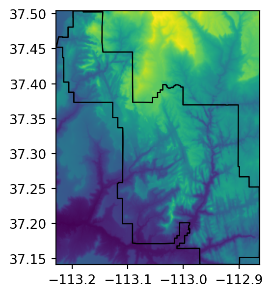
zion = zion.to_crs(src_srtm.crs)To mask the image, i.e., convert all pixels which do not intersect with the zion polygon to ‘No Data’, we use the rasterio.mask.mask function.
out_image_mask, out_transform_mask = rasterio.mask.mask(
    src_srtm,
    zion.geometry,
    crop=False,
    nodata=9999
)
Note that we need to choose and specify a ‘No Data’ value, within the valid range according to the data type. Since srtm.tif is of type uint16 (how can we check?1), we choose 9999 (a positive integer that is guaranteed not to occur in the raster). Also note that rasterio does not directly support geopandas data structures, so we need to pass a ‘collection’ of shapely geometries: a GeoSeries (see above) or a list of shapely geometries (see next example) both work. The output consists of two objects. The first one is the out_image array with the masked values.
out_image_maskarray([[[9999, 9999, 9999, ..., 9999, 9999, 9999],
[9999, 9999, 9999, ..., 9999, 9999, 9999],
[9999, 9999, 9999, ..., 9999, 9999, 9999],
...,
[9999, 9999, 9999, ..., 9999, 9999, 9999],
[9999, 9999, 9999, ..., 9999, 9999, 9999],
[9999, 9999, 9999, ..., 9999, 9999, 9999]]], dtype=uint16)The second one is a new transformation matrix out_transform.
out_transform_maskAffine(0.0008333333332777796, 0.0, -113.23958321278403,
0.0, -0.0008333333332777843, 37.512916763165805)Note that masking (without cropping!) does not modify the raster extent. Therefore, the new transform is identical to the original (src_srtm.transform).
Unfortunately, the out_image and out_transform objects do not contain any information indicating that 9999 represents ‘No Data’. To associate the information with the raster, we must write it to file along with the corresponding metadata. For example, to write the masked raster to file, we first need to modify the ‘No Data’ setting in the metadata.
dst_kwargs = src_srtm.meta
dst_kwargs.update(nodata=9999)
dst_kwargs
{'driver': 'GTiff',
'dtype': 'uint16',
'nodata': 9999,
'width': 465,
'height': 457,
'count': 1,
'crs': CRS.from_epsg(4326),
'transform': Affine(0.0008333333332777796, 0.0, -113.23958321278403,
0.0, -0.0008333333332777843, 37.512916763165805)}Then we can write the masked raster to file with the updated metadata object.
new_dataset = rasterio.open('output/srtm_masked.tif', 'w', **dst_kwargs)
new_dataset.write(out_image_mask)
new_dataset.close()
Now we can re-import the raster and check that the ‘No Data’ value is correctly set.
src_srtm_mask = rasterio.open('output/srtm_masked.tif')The .meta property contains the nodata entry. Now, any relevant operation (such as plotting, see Figure 5.2 (b)) will take ‘No Data’ into account.
src_srtm_mask.meta{'driver': 'GTiff',
'dtype': 'uint16',
'nodata': 9999.0,
'width': 465,
'height': 457,
'count': 1,
'crs': CRS.from_epsg(4326),
'transform': Affine(0.0008333333332777796, 0.0, -113.23958321278403,
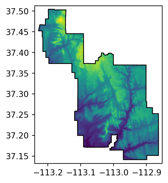
0.0, -0.0008333333332777843, 37.512916763165805)}The related operation, cropping, reduces the raster extent to the extent of the vector layer:
- To crop and mask, we can use
rasterio.mask.mask, same as above for masking, while settingcrop=True(Figure 5.2 (d)) - To just crop, without masking, we can derive the bounding box polygon of the vector layer, and then crop using that polygon, also combined with
crop=True(Figure 5.2 (c))
For the example of cropping only, the extent polygon of zion can be obtained as a shapely geometry object using .union_all().envelope (Figure 5.1).
bb = zion.union_all().envelope
bb
'Polygon' geometry of the zion layer
The extent can now be used for masking. Here, we are also using the all_touched=True option, so that pixels which are partially overlapping with the extent are also included in the output.
out_image_crop, out_transform_crop = rasterio.mask.mask(
    src_srtm,
    [bb],
    crop=True,
    all_touched=True,
    nodata=9999
)
In the case of cropping, there is no particular reason to write the result to file for easier plotting, such as in the other two examples, since there are no ‘No Data’ values (Figure 5.2 (c)).
Note
As mentioned above, rasterio functions typically accept vector geometries in the form of lists of shapely objects. GeoSeries are conceptually very similar, and also accepted. However, even an individual geometry has to be in a list, which is why we pass [bb], and not bb, in the above rasterio.mask.mask function call (the latter would raise an error).
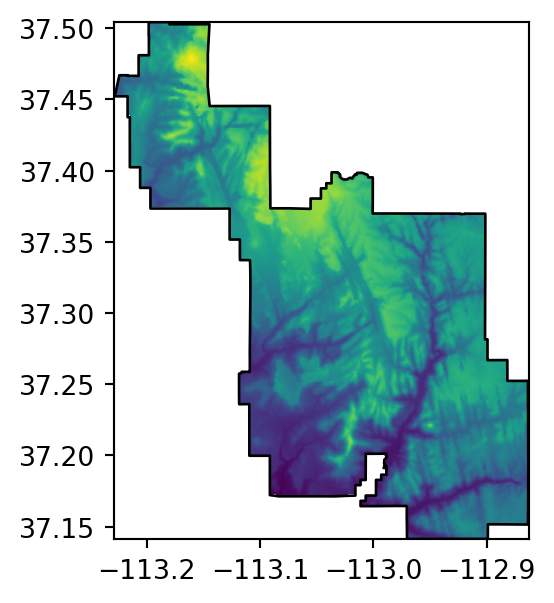
Finally, the third example is where we perform both crop and mask operations, using rasterio.mask.mask with crop=True passing zion.geometry.
out_image_mask_crop, out_transform_mask_crop = rasterio.mask.mask(
    src_srtm,
    zion.geometry,
    crop=True,
    nodata=9999
)
When writing the result to a file, it is here crucial to update the transform and dimensions, since they were modified as a result of cropping. Also note that out_image_mask_crop is a three-dimensional array (even though it has one band in this case), so the number of rows and columns are in .shape[1] and .shape[2] (rather than .shape[0] and .shape[1]), respectively.
dst_kwargs = src_srtm.meta
dst_kwargs.update({
    'nodata': 9999,
    'transform': out_transform_mask_crop,
    'width': out_image_mask_crop.shape[2],
    'height': out_image_mask_crop.shape[1]
})
new_dataset = rasterio.open(
    'output/srtm_masked_cropped.tif',
    'w',
    **dst_kwargs
)
new_dataset.write(out_image_mask_crop)
new_dataset.close()
Let’s also create a file connection to the newly created file srtm_masked_cropped.tif in order to plot it (Figure 5.2 (d)).
src_srtm_mask_crop = rasterio.open('output/srtm_masked_cropped.tif')Figure 5.2 shows the original raster, and the three masking and/or cropping results.
# Original
fig, ax = plt.subplots(figsize=(3.5, 3.5))
rasterio.plot.show(src_srtm, ax=ax)
zion.plot(ax=ax, color='none', edgecolor='black');
# Masked
fig, ax = plt.subplots(figsize=(3.5, 3.5))
rasterio.plot.show(src_srtm_mask, ax=ax)
zion.plot(ax=ax, color='none', edgecolor='black');
# Cropped
fig, ax = plt.subplots(figsize=(3.5, 3.5))
rasterio.plot.show(out_image_crop, transform=out_transform_crop, ax=ax)
zion.plot(ax=ax, color='none', edgecolor='black');
# Masked+Cropped
fig, ax = plt.subplots(figsize=(3.5, 3.5))
rasterio.plot.show(src_srtm_mask_crop, ax=ax)
zion.plot(ax=ax, color='none', edgecolor='black');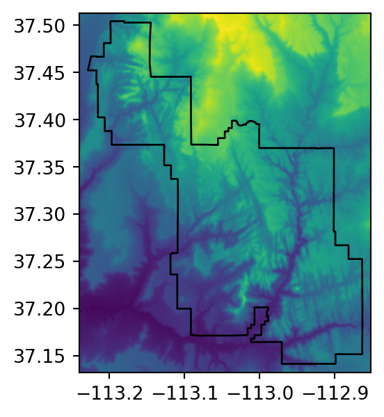
5.3 Raster extraction
Raster extraction is the process of identifying and returning the values associated with a ‘target’ raster at specific locations, based on a (typically vector) geographic ‘selector’ object. The reverse of raster extraction—assigning raster cell values based on vector objects—is rasterization, described in Section 5.4.
In the following examples, we use a package called rasterstats, which is specifically aimed at extracting raster values:
- To points (Section 5.3.1) or to lines (Section 5.3.2), via the
rasterstats.point_queryfunction - To polygons (Section 5.3.3), via the
rasterstats.zonal_statsfunction
5.3.1 Extraction to points
The simplest type of raster extraction is getting the values of raster cells at specific points. To demonstrate extraction to points, we will use zion_points, which contains a sample of 30 locations within the Zion National Park (Figure 5.3).
fig, ax = plt.subplots()
rasterio.plot.show(src_srtm, ax=ax)
zion_points.plot(ax=ax, color='black', edgecolor='white');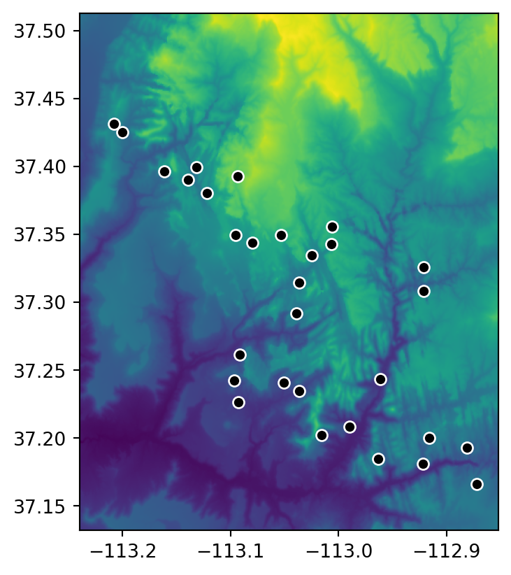
The following expression extracts elevation values from srtm.tif according to zion_points, using rasterstats.point_query.
result1 = rasterstats.point_query(
    zion_points,
    src_srtm.read(1),
    nodata = src_srtm.nodata,
    affine = src_srtm.transform,
    interpolate='nearest'
)
The first two arguments are the vector layer and the array with raster values. The nodata and affine arguments are used to align the array values into the CRS, and to correctly treat ‘No Data’ flags. Finally, the interpolate argument controls the way that the cell values are assigned to the point; interpolate='nearest' typically makes more sense, as opposed to the other option interpolate='bilinear' which is the default.
Alternatively, we can pass a raster file path to rasterstats.point_query, in which case nodata and affine are not necessary, as the function can understand those properties directly from the raster file.
result2 = rasterstats.point_query(
    zion_points,
    'data/srtm.tif',
    interpolate='nearest'
)
Either way, the resulting object is a list of raster values, corresponding to zion_points. For example, here are the elevations of the first five points.
result1[:5][1802, 2433, 1886, 1370, 1452]To get a GeoDataFrame with the original points geometries (and other attributes, if any), as well as the extracted raster values, we can assign the extraction result into a new column. As you can see, both approaches give the same result.
zion_points['elev1'] = result1
zion_points['elev2'] = result2
zion_points| geometry | elev1 | elev2 | |
|---|---|---|---|
| 0 | POINT (-112.91587 37.20013) | 1802 | 1802 |
| 1 | POINT (-113.09369 37.39263) | 2433 | 2433 |
| 2 | POINT (-113.02462 37.33466) | 1886 | 1886 |
| ... | ... | ... | ... |
| 27 | POINT (-113.03655 37.23446) | 1372 | 1372 |
| 28 | POINT (-113.13933 37.39004) | 1905 | 1905 |
| 29 | POINT (-113.09677 37.24237) | 1574 | 1574 |
30 rows × 3 columns
The function supports extracting from just one raster band at a time. When passing an array, we can read the required band (as in, .read(1), .read(2), etc.). When passing a raster file path, we can set the band using the band_num argument (the default being band_num=1).
5.3.2 Extraction to lines
Raster extraction is also applicable with line selectors. The typical line extraction algorithm is to extract one value for each raster cell touched by a line. However, this particular approach is not recommended to obtain values along the transects, as it is hard to get the correct distance between each pair of extracted raster values.
For line extraction, a better approach is to split the line into many points (at equal distances along the line) and then extract the values for these points using the ‘extraction to points’ technique (Section 5.3.1). To demonstrate this, the code below creates (see Section 1.2 for recap) zion_transect, a straight line going from northwest to southeast of the Zion National Park.
coords = [[-113.2, 37.45], [-112.9, 37.2]]
zion_transect = shapely.LineString(coords)
print(zion_transect)
LINESTRING (-113.2 37.45, -112.9 37.2)The utility of extracting heights from a linear selector is illustrated by imagining that you are planning a hike. The method demonstrated below provides an ‘elevation profile’ of the route (the line does not need to be straight), useful for estimating how long it will take due to long climbs.
First, we need to create a layer consisting of points along our line (zion_transect), at specified intervals (e.g., 250). To do that, we need to transform the line into a projected CRS (so that we work with true distances, in \(m\)), such as UTM. This requires going through a GeoSeries, as shapely geometries have no CRS definition nor concept of reprojection (see Section 1.2.6).
zion_transect_utm = gpd.GeoSeries(zion_transect, crs=4326).to_crs(32612)
zion_transect_utm = zion_transect_utm.iloc[0]
The printout of the new geometry shows this is still a straight line between two points, only with coordinates in a projected CRS.
print(zion_transect_utm)LINESTRING (305399.67208180577 4147066.650206682, 331380.8917453843 4118750.0947884847)Next, we need to calculate the distances, along the line, where points are going to be generated. We do this using np.arange. The result is a numeric sequence starting at 0, going up to line .length, in steps of 250 (\(m\)).
distances = np.arange(0, zion_transect_utm.length, 250)
distances[:7]  ## First 7 distance cutoff points
array([ 0., 250., 500., 750., 1000., 1250., 1500.])The distance cutoffs are used to sample (‘interpolate’) points along the line. The shapely .interpolate method is used to generate the points, which then are reprojected back to the geographic CRS of the raster (EPSG:4326).
zion_transect_pnt = [zion_transect_utm.interpolate(d) for d in distances]
zion_transect_pnt = gpd.GeoSeries(zion_transect_pnt, crs=32612) \
    .to_crs(src_srtm.crs)
zion_transect_pnt
0 POINT (-113.2 37.45)
1 POINT (-113.19804 37.44838)
2 POINT (-113.19608 37.44675)
...
151 POINT (-112.90529 37.20443)
152 POINT (-112.90334 37.2028)
153 POINT (-112.9014 37.20117)
Length: 154, dtype: geometryFinally, we extract the elevation values for each point in our transect and combine the information with zion_transect_pnt (after ‘promoting’ it to a GeoDataFrame, to accommodate extra attributes), using the point extraction method shown earlier (Section 5.3.1). We also attach the respective distance cutoff points distances.
result = rasterstats.point_query(
    zion_transect_pnt,
    src_srtm.read(1),
    nodata = src_srtm.nodata,
    affine = src_srtm.transform,
    interpolate='nearest'
)
zion_transect_pnt = gpd.GeoDataFrame(geometry=zion_transect_pnt)
zion_transect_pnt['dist'] = distances
zion_transect_pnt['elev'] = result
zion_transect_pnt| geometry | dist | elev | |
|---|---|---|---|
| 0 | POINT (-113.2 37.45) | 0.0 | 2001 |
| 1 | POINT (-113.19804 37.44838) | 250.0 | 2037 |
| 2 | POINT (-113.19608 37.44675) | 500.0 | 1949 |
| ... | ... | ... | ... |
| 151 | POINT (-112.90529 37.20443) | 37750.0 | 1837 |
| 152 | POINT (-112.90334 37.2028) | 38000.0 | 1841 |
| 153 | POINT (-112.9014 37.20117) | 38250.0 | 1819 |
154 rows × 3 columns
The information in zion_transect_pnt, namely the 'dist' and 'elev' attributes, can now be used to draw an elevation profile, as illustrated in Figure 5.4.
# Raster and a line transect
fig, ax = plt.subplots()
rasterio.plot.show(src_srtm, ax=ax)
gpd.GeoSeries(zion_transect).plot(ax=ax, color='black')
zion.plot(ax=ax, color='none', edgecolor='white');
# Elevation profile
fig, ax = plt.subplots()
zion_transect_pnt.set_index('dist')['elev'].plot(ax=ax)
ax.set_xlabel('Distance (m)')
ax.set_ylabel('Elevation (m)');5.3.3 Extraction to polygons
The final type of geographic vector object for raster extraction is polygons. Like lines, polygons tend to return many raster values per vector geometry. For continuous rasters (Figure 5.5 (a)), we typically want to generate summary statistics for raster values per polygon, for example to characterize a single region or to compare many regions. The generation of raster summary statistics, by polygons, is demonstrated in the code below using rasterstats.zonal_stats, which creates a list of summary statistics (in this case a list of length 1, since there is just one polygon).
result = rasterstats.zonal_stats(
    zion,
    src_srtm.read(1),
    nodata = src_srtm.nodata,
    affine = src_srtm.transform,
    stats = ['mean', 'min', 'max']
)
result
[{'min': 1122.0, 'max': 2661.0, 'mean': 1818.211830154405}]
Note
rasterstats.zonal_stats, just like rasterstats.point_query (Section 5.3.1), supports raster input as file paths, rather than arrays plus nodata and affine arguments.
Transformation of the list to a DataFrame (e.g., to attach the derived attributes to the original polygon layer), is straightforward with the pd.DataFrame constructor.
pd.DataFrame(result)| min | max | mean | |
|---|---|---|---|
| 0 | 1122.0 | 2661.0 | 1818.21183 |
Because there is only one polygon in the example, a DataFrame with a single row is returned. However, if zion was composed of more than one polygon, we would accordingly get more rows in the DataFrame. The result provides useful summaries, for example that the maximum height in the park is 2661 \(m\) above see level.
Note the stats argument, where we determine what type of statistics are calculated per polygon. Possible values other than 'mean', 'min', and 'max' include:
'count'—The number of valid (i.e., excluding ‘No Data’) pixels'nodata'—The number of pixels with ‘No Data’'majority'—The most frequently occurring value'median'—The median value
See the documentation of rasterstats.zonal_stats for the complete list. Additionally, the rasterstats.zonal_stats function accepts user-defined functions for calculating any custom statistics.
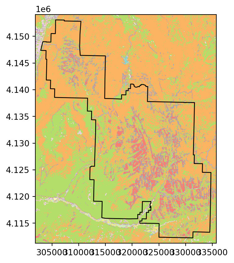
To count occurrences of categorical raster values within polygons (Figure 5.5 (b)), we can use masking (Section 5.2) combined with np.unique, as follows.
out_image, out_transform = rasterio.mask.mask(
    src_nlcd,
    zion.geometry.to_crs(src_nlcd.crs),
    crop=False,
    nodata=src_nlcd.nodata
)
counts = np.unique(out_image, return_counts=True)
counts
(array([ 2, 3, 4, 5, 6, 7, 8, 255], dtype=uint8),
array([ 4205, 98285, 298299, 203701, 235, 62, 679, 852741]))According to the result, for example, the value 2 (‘Developed’ class) appears in 4205 pixels within the Zion polygon.
Figure 5.5 illustrates the two types of raster extraction to polygons described above.
# Continuous raster
fig, ax = plt.subplots()
rasterio.plot.show(src_srtm, ax=ax)
zion.plot(ax=ax, color='none', edgecolor='black');
# Categorical raster
fig, ax = plt.subplots()
rasterio.plot.show(src_nlcd, ax=ax, cmap='Set3')
zion.to_crs(src_nlcd.crs).plot(ax=ax, color='none', edgecolor='black');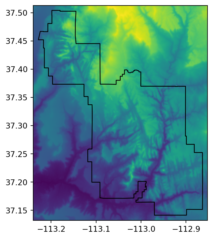
5.4 Rasterization
Rasterization is the conversion of vector objects into their representation in raster objects. Usually, the output raster is used for quantitative analysis (e.g., analysis of terrain) or modeling. As we saw in Chapter 1, the raster data model has some characteristics that make it conducive to certain methods. Furthermore, the process of rasterization can help simplify datasets because the resulting values all have the same spatial resolution: rasterization can be seen as a special type of geographic data aggregation.
The rasterio package contains the rasterio.features.rasterize function for doing this work. To make it happen, we need to have the ‘template’ grid definition, i.e., the ‘template’ raster defining the extent, resolution and CRS of the output, in the out_shape (the output dimensions) and transform (the transformation matrix) arguments of rasterio.features.rasterize. In case we have an existing template raster, we simply need to query its .shape and .transform. On the other hand, if we need to create a custom template, e.g., covering the vector layer extent with specified resolution, there is some extra work to calculate both of these objects (see next example).
As for the vector geometries and their associated values, the rasterio.features.rasterize function requires the input vector shapes in the form of an iterable object of geometry,value pairs, where:
geometryis the given geometry (shapely geometry object)valueis the value to be ‘burned’ into pixels coinciding with the geometry (intorfloat)
Furthermore, we define how to deal with multiple values burned into the same pixel, using the merge_alg parameter. The default merge_alg=rasterio.enums.MergeAlg.replace means that ‘later’ values replace ‘earlier’ ones, i.e., the pixel gets the ‘last’ burned value. The other option merge_alg=rasterio.enums.MergeAlg.add means that burned values are summed, i.e., the pixel gets the sum of all burned values.
When rasterizing lines and polygons, we also have the choice between two pixel-matching algorithms. The default, all_touched=False, implies pixels that are selected by Bresenham’s line algorithm2 (for lines) or pixels whose center is within the polygon (for polygons). The other option all_touched=True, as the name suggests, implies that all pixels intersecting with the geometry are matched.
Finally, we can set the fill value, which is the value that ‘unaffected’ pixels get, with fill=0 being the default.
How the rasterio.features.rasterize function works with all of these various parameters will be made clear in the next examples.
The geographic resolution of the ‘template’ raster has a major impact on the results: if it is too low (cell size is too large), the result may miss the full geographic variability of the vector data; if it is too high, computational times may be excessive. There are no simple rules to follow when deciding an appropriate geographic resolution, which is heavily dependent on the intended use of the results. Often the target resolution is imposed on the user, for example when the output of rasterization needs to be aligned to an existing raster.
Depending on the input data, rasterization typically takes one of two forms which we demonstrate next:
- in point rasterization (Section 5.4.1), we typically choose how to treat multiple points: either to summarize presence/absence, point count, or summed attribute values (Figure 5.6)
- in line and polygon rasterization (Section 5.4.2), there are typically no such ‘overlaps’ and we simply ‘burn’ attribute values, or fixed values, into pixels coinciding with the given geometries (Figure 5.7)
5.4.1 Rasterizing points
To demonstrate point rasterization, we will prepare a ‘template’ raster that has the same extent and CRS as the input vector data cycle_hire_osm_projected (a dataset on cycle hire points in London, illustrated in Figure 5.6 (a)) and a spatial resolution of 1000 \(m\). To do that, we first take our point layer and transform it to a projected CRS.
cycle_hire_osm_projected = cycle_hire_osm.to_crs(27700)Next, we calculate the out_shape and transform of the template raster. To calculate the transform, we combine the top-left corner of the cycle_hire_osm_projected bounding box with the required resolution (e.g., 1000 \(m\)).
bounds = cycle_hire_osm_projected.total_bounds
res = 1000
transform = rasterio.transform.from_origin(
    west=bounds[0],
    north=bounds[3],
    xsize=res,
    ysize=res
)
transform
Affine(1000.0, 0.0, np.float64(523038.61452275474),
0.0, -1000.0, np.float64(184971.40854297992))To calculate the out_shape, we divide the x-axis and y-axis extent by the resolution, taking the ceiling of the results.
rows = math.ceil((bounds[3] - bounds[1]) / res)
cols = math.ceil((bounds[2] - bounds[0]) / res)
shape = (rows, cols)
shape
(11, 16)Finally, we are ready to rasterize. As mentioned above, point rasterization can be a very flexible operation: the results depend not only on the nature of the template raster, but also on the pixel ‘activation’ method, namely the way we deal with multiple points matching the same pixel.
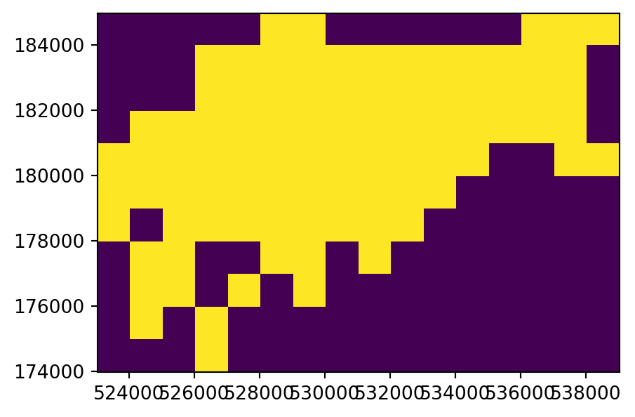
To illustrate this flexibility, we will try three different approaches to point rasterization (Figure 5.6 (b)-(d)). First, we create a raster representing the presence or absence of cycle hire points (known as presence/absence rasters). In this case, we transfer the value of 1 to all pixels where at least one point falls in. In the rasterio framework, we use the rasterio.features.rasterize function, which requires an iterable object of geometry,value pairs. In this first example, we transform the point GeoDataFrame into a list of shapely geometries and the (fixed) value of 1, using list comprehension, as follows. The first five elements of the list are hereby printed to illustrate its structure.
g = [(g, 1) for g in cycle_hire_osm_projected.geometry]
g[:5]
[(<POINT (532353.838 182857.655)>, 1),
(<POINT (529848.35 183337.175)>, 1),
(<POINT (530635.62 182608.992)>, 1),
(<POINT (532540.398 182495.756)>, 1),
(<POINT (530432.094 182906.846)>, 1)]The list of geometry,value pairs is passed to rasterio.features.rasterize, along with the out_shape and transform which define the raster template. The result ch_raster1 is an ndarray with the burned values of 1 where the pixel coincides with at least one point, and 0 in ‘unaffected’ pixels. Note that merge_alg=rasterio.enums.MergeAlg.replace (the default) is used here, which means that a pixel gets 1 when one or more points fall in it, or keeps the original 0 value otherwise.
ch_raster1 = rasterio.features.rasterize(
    shapes=g,
    out_shape=shape,
    transform=transform
)
ch_raster1
array([[0, 0, 0, 0, 0, 1, 1, 0, 0, 0, 0, 0, 0, 1, 1, 1],
[0, 0, 0, 1, 1, 1, 1, 1, 1, 1, 1, 1, 1, 1, 1, 0],
[0, 0, 0, 1, 1, 1, 1, 1, 1, 1, 1, 1, 1, 1, 1, 0],
[0, 1, 1, 1, 1, 1, 1, 1, 1, 1, 1, 1, 1, 1, 1, 0],
[1, 1, 1, 1, 1, 1, 1, 1, 1, 1, 1, 1, 0, 0, 1, 1],
[1, 1, 1, 1, 1, 1, 1, 1, 1, 1, 1, 0, 0, 0, 0, 0],
[1, 0, 1, 1, 1, 1, 1, 1, 1, 1, 0, 0, 0, 0, 0, 0],
[0, 1, 1, 0, 0, 1, 1, 0, 1, 0, 0, 0, 0, 0, 0, 0],
[0, 1, 1, 0, 1, 0, 1, 0, 0, 0, 0, 0, 0, 0, 0, 0],
[0, 1, 0, 1, 0, 0, 0, 0, 0, 0, 0, 0, 0, 0, 0, 0],
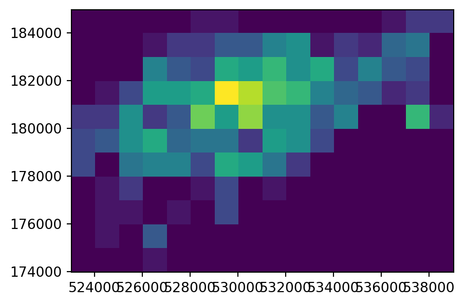
[0, 0, 0, 1, 0, 0, 0, 0, 0, 0, 0, 0, 0, 0, 0, 0]], dtype=uint8)In our second variant of point rasterization, we count the number of bike hire stations. To do that, we use the fixed value of 1 (same as in the last example), but this time combined with the merge_alg=rasterio.enums.MergeAlg.add argument. That way, multiple values burned into the same pixel are summed, rather than replaced keeping last (which is the default). The new output, ch_raster2, shows the number of cycle hire points in each grid cell.
g = [(g, 1) for g in cycle_hire_osm_projected.geometry]
ch_raster2 = rasterio.features.rasterize(
    shapes=g,
    out_shape=shape,
    transform=transform,
    merge_alg=rasterio.enums.MergeAlg.add
)
ch_raster2
array([[ 0, 0, 0, 0, 0, 1, 1, 0, 0, 0, 0, 0, 0, 1, 3, 3],
[ 0, 0, 0, 1, 3, 3, 5, 5, 8, 9, 1, 3, 2, 6, 7, 0],
[ 0, 0, 0, 8, 5, 4, 11, 10, 12, 9, 11, 4, 8, 5, 4, 0],
[ 0, 1, 4, 10, 10, 11, 18, 16, 13, 12, 8, 6, 5, 2, 3, 0],
[ 3, 3, 9, 3, 5, 14, 10, 15, 9, 9, 5, 8, 0, 0, 12, 2],
[ 4, 5, 9, 11, 6, 7, 7, 3, 10, 9, 4, 0, 0, 0, 0, 0],
[ 4, 0, 7, 8, 8, 4, 11, 10, 7, 3, 0, 0, 0, 0, 0, 0],
[ 0, 1, 3, 0, 0, 1, 4, 0, 1, 0, 0, 0, 0, 0, 0, 0],
[ 0, 1, 1, 0, 1, 0, 4, 0, 0, 0, 0, 0, 0, 0, 0, 0],
[ 0, 1, 0, 5, 0, 0, 0, 0, 0, 0, 0, 0, 0, 0, 0, 0],
[ 0, 0, 0, 1, 0, 0, 0, 0, 0, 0, 0, 0, 0, 0, 0, 0]],
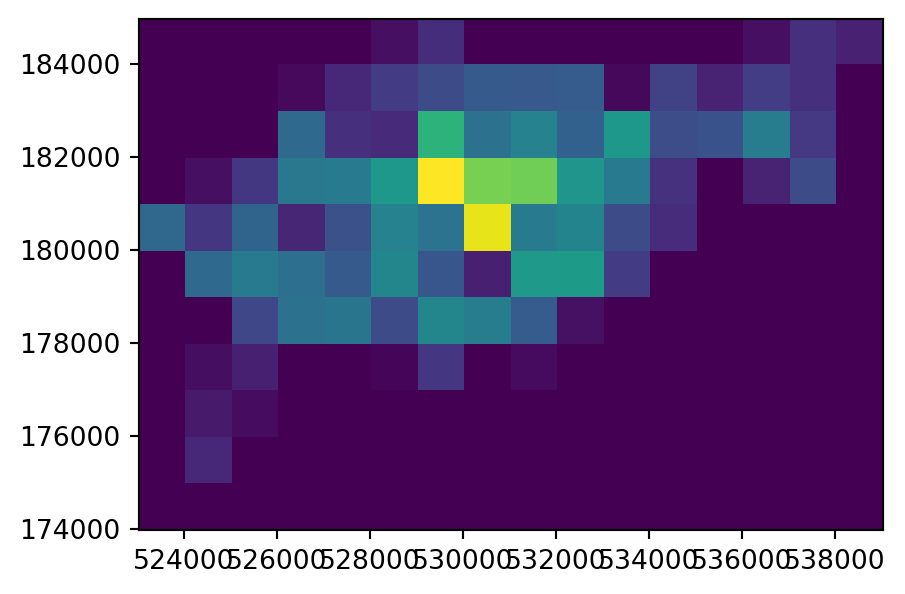
dtype=uint8)The cycle hire locations have different numbers of bicycles described by the capacity variable, raising the question, what is the capacity in each grid cell? To calculate that, in our third point rasterization variant we sum the field ('capacity') rather than the fixed values of 1. This requires using a more complex list comprehension expression, where we also (1) extract both geometries and the attribute of interest, and (2) filter out ‘No Data’ values, which can be done as follows. You are invited to run the separate parts to see how this works; the important point is that, in the end, we get the list g with the geometry,value pairs to be burned, only that the value is now variable, rather than fixed, among points.
g = [(g, v) for g, v in cycle_hire_osm_projected[['geometry', 'capacity']] \
        .dropna(subset='capacity')
        .to_numpy() \
        .tolist()]
g[:5]
[(<POINT (532353.838 182857.655)>, 14.0),
(<POINT (530635.62 182608.992)>, 11.0),
(<POINT (532620.775 181944.736)>, 20.0),
(<POINT (527891.578 181374.392)>, 6.0),
(<POINT (530399.064 181205.925)>, 17.0)]Now we rasterize the points, again using merge_alg=rasterio.enums.MergeAlg.add to sum the capacity values per pixel.
ch_raster3 = rasterio.features.rasterize(
    shapes=g,
    out_shape=shape,
    transform=transform,
    merge_alg=rasterio.enums.MergeAlg.add
)
ch_raster3
array([[ 0., 0., 0., 0., 0., 11., 34., 0., 0., 0., 0.,
0., 0., 11., 35., 24.],
[ 0., 0., 0., 7., 30., 46., 60., 73., 72., 75., 6.,
50., 25., 47., 36., 0.],
[ 0., 0., 0., 89., 36., 31., 167., 97., 115., 80., 138.,
61., 65., 109., 43., 0.],
[ 0., 11., 42., 104., 108., 138., 259., 206., 203., 135., 107.,
37., 0., 25., 60., 0.],
[ 88., 41., 83., 28., 64., 115., 99., 249., 107., 117., 60.,
33., 0., 0., 0., 0.],
[ 0., 89., 107., 95., 73., 119., 69., 23., 140., 141., 46.,
0., 0., 0., 0., 0.],
[ 0., 0., 55., 97., 101., 59., 119., 109., 75., 12., 0.,
0., 0., 0., 0., 0.],
[ 0., 10., 23., 0., 0., 5., 41., 0., 8., 0., 0.,
0., 0., 0., 0., 0.],
[ 0., 19., 9., 0., 0., 0., 0., 0., 0., 0., 0.,
0., 0., 0., 0., 0.],
[ 0., 29., 0., 0., 0., 0., 0., 0., 0., 0., 0.,
0., 0., 0., 0., 0.],
[ 0., 0., 0., 0., 0., 0., 0., 0., 0., 0., 0.,
0., 0., 0., 0., 0.]], dtype=float32)The result ch_raster3 shows the total capacity of cycle hire points in each grid cell.
The input point layer cycle_hire_osm_projected and the three variants of rasterizing it ch_raster1, ch_raster2, and ch_raster3 are shown in Figure 5.6.
# Input points
fig, ax = plt.subplots()
cycle_hire_osm_projected.plot(column='capacity', ax=ax);
# Presence/Absence
fig, ax = plt.subplots()
rasterio.plot.show(ch_raster1, transform=transform, ax=ax);
# Point counts
fig, ax = plt.subplots()
rasterio.plot.show(ch_raster2, transform=transform, ax=ax);
# Summed attribute values
fig, ax = plt.subplots()
rasterio.plot.show(ch_raster3, transform=transform, ax=ax);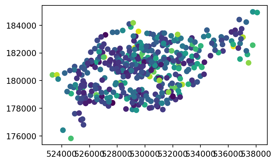
5.4.2 Rasterizing lines and polygons
Another dataset based on California’s polygons and borders (created below) illustrates rasterization of lines. There are three preliminary steps. First, we subset the California polygon.
california = us_states[us_states['NAME'] == 'California']
california| GEOID | NAME | ... | total_pop_15 | geometry | |
|---|---|---|---|---|---|
| 26 | 06 | California | ... | 38421464.0 | MULTIPOLYGON (((-118.60338 33.4... |
1 rows × 7 columns
Second, we ‘cast’ the polygon into a 'MultiLineString' geometry, using the .boundary property that GeoSeries and DataFrames have.
california_borders = california.boundary
california_borders
26 MULTILINESTRING ((-118.60338 33...
dtype: geometryThird, we create the transform and shape describing our template raster, with a resolution of 0.5 degree, using the same approach as in Section 5.4.1.
bounds = california_borders.total_bounds
res = 0.5
transform = rasterio.transform.from_origin(
west=bounds[0],
north=bounds[3],
xsize=res,
ysize=res
)
rows = math.ceil((bounds[3] - bounds[1]) / res)
cols = math.ceil((bounds[2] - bounds[0]) / res)
shape = (rows, cols)
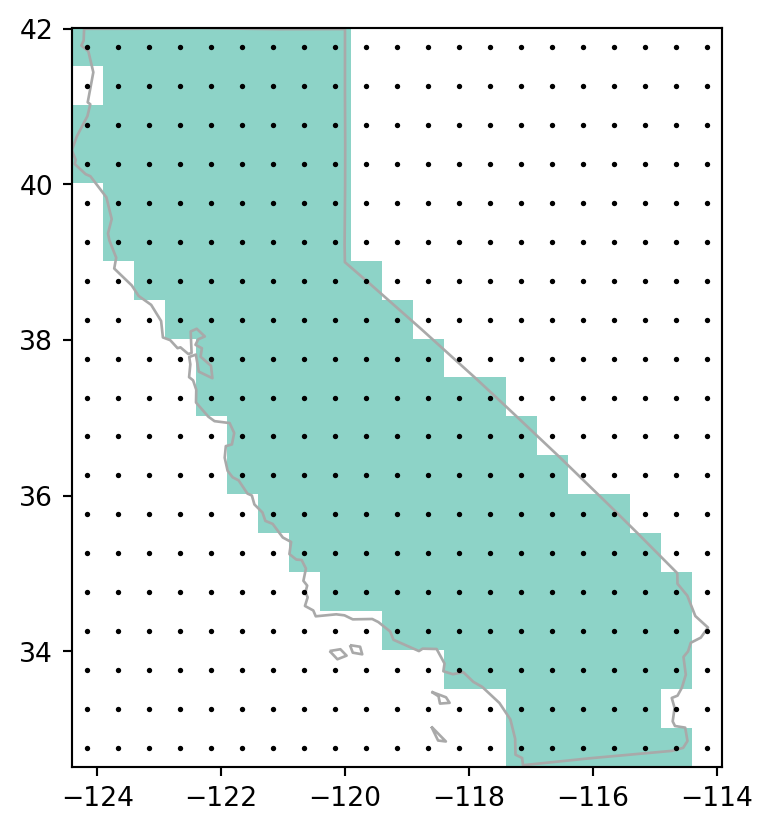
shape(19, 21)Finally, we rasterize california_borders based on the calculated template’s shape and transform. When considering line or polygon rasterization, one useful additional argument is all_touched. By default it is False, but when changed to True—all cells that are touched by a line or polygon border get a value. Line rasterization with all_touched=True is demonstrated in the code below (Figure 5.7, left). We are also using fill=np.nan to set ‘background’ values to ‘No Data’.
california_raster1 = rasterio.features.rasterize(
    [(g, 1) for g in california_borders],
    out_shape=shape,
    transform=transform,
    all_touched=True,
    fill=np.nan,
    dtype=np.float64
)
Compare it to polygon rasterization, with all_touched=False (the default), which selects only raster cells whose centroids are inside the selector polygon, as illustrated in Figure 5.7 (right).
california_raster2 = rasterio.features.rasterize(
    [(g, 1) for g in california.geometry],
    out_shape=shape,
    transform=transform,
    fill=np.nan,
    dtype=np.float64
)
To illustrate which raster pixels are actually selected as part of rasterization, we also show them as points. This also requires the following code section to calculate the points, which we explain in Section 5.5.
height = california_raster1.shape[0]
width = california_raster1.shape[1]
cols, rows = np.meshgrid(np.arange(width), np.arange(height))
x, y = rasterio.transform.xy(transform, rows, cols)
x = np.array(x).flatten()
y = np.array(y).flatten()
z = california_raster1.flatten()
geom = gpd.points_from_xy(x, y, crs=california.crs)
pnt = gpd.GeoDataFrame(data={'value':z}, geometry=geom)
pnt| value | geometry | |
|---|---|---|
| 0 | 1.0 | POINT (-124.15959 41.75952) |
| 1 | 1.0 | POINT (-123.65959 41.75952) |
| 2 | 1.0 | POINT (-123.15959 41.75952) |
| ... | ... | ... |
| 396 | 1.0 | POINT (-115.15959 32.75952) |
| 397 | 1.0 | POINT (-114.65959 32.75952) |
| 398 | NaN | POINT (-114.15959 32.75952) |
399 rows × 2 columns
Figure 5.7 shows the input vector layer, the rasterization results, and the points pnt.
# Line rasterization
fig, ax = plt.subplots()
rasterio.plot.show(california_raster1, transform=transform, ax=ax, cmap='Set3')
gpd.GeoSeries(california_borders).plot(ax=ax, edgecolor='darkgrey', linewidth=1)
pnt.plot(ax=ax, color='black', markersize=1);
# Polygon rasterization
fig, ax = plt.subplots()
rasterio.plot.show(california_raster2, transform=transform, ax=ax, cmap='Set3')
california.plot(ax=ax, color='none', edgecolor='darkgrey', linewidth=1)
pnt.plot(ax=ax, color='black', markersize=1);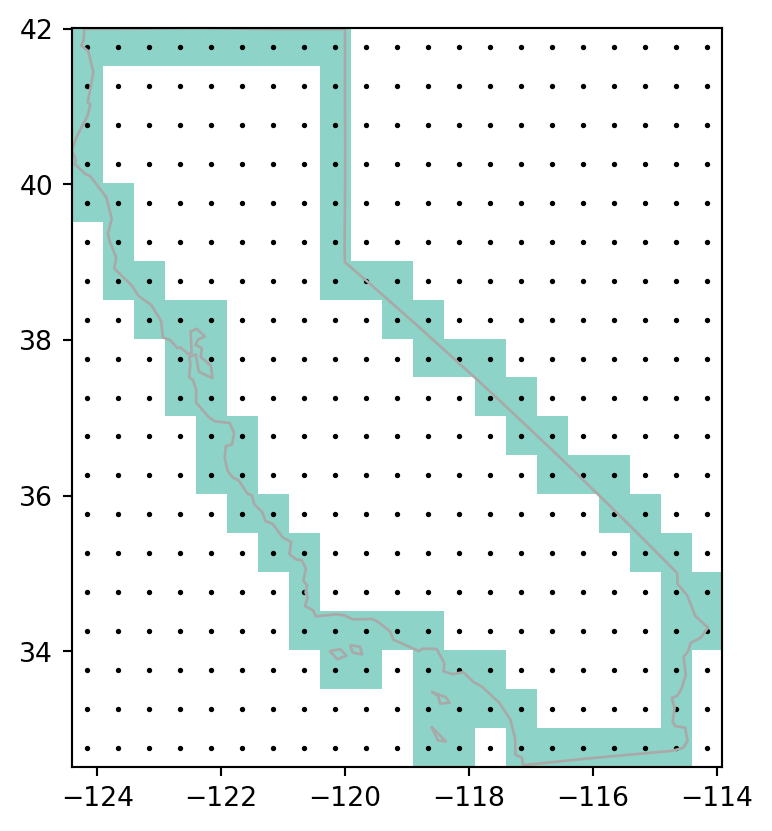
all_touched=True
all_touched=False
5.5 Spatial vectorization
Spatial vectorization is the counterpart of rasterization (Section 5.4). It involves converting spatially continuous raster data into spatially discrete vector data such as points, lines, or polygons. There are three standard methods to convert a raster to a vector layer, which we cover next:
- Raster to polygons (Section 5.5.1)—converting raster cells to rectangular polygons, representing pixel areas
- Raster to points (Section 5.5.2)—converting raster cells to points, representing pixel centroids
- Raster to contours (Section 5.5.3)
Let us demonstrate all three in the given order.
5.5.1 Raster to polygons
The rasterio.features.shapes gives access to raster pixels as polygon geometries, along with the associated raster values. The returned object is a generator (see note in Section 3.3.1), yielding geometry,value pairs.
For example, the following expression returns a generator named shapes, referring to the pixel polygons.
shapes = rasterio.features.shapes(rasterio.band(src_grain, 1))
shapes
<generator object shapes at 0x7f9a463abcd0>We can generate all shapes at once into a list named pol with list(shapes).
pol = list(shapes)Each element in pol is a tuple of length 2, containing the GeoJSON-like dict—representing the polygon geometry and the value of the pixel(s) which comprise the polygon. For example, here is the first element of pol.
pol[0]({'type': 'Polygon',
'coordinates': [[(-1.5, 1.5),
(-1.5, 1.0),
(-1.0, 1.0),
(-1.0, 1.5),
(-1.5, 1.5)]]},
1.0)
Note
Note that, when transforming a raster cell into a polygon, five-coordinate pairs need to be kept in memory to represent its geometry (explaining why rasters are often fast compared with vectors!).
To transform the list coming out of rasterio.features.shapes into the familiar GeoDataFrame, we need few more steps of data reshaping. First, we apply the shapely.geometry.shape function to go from a list of GeoJSON-like dicts to a list of shapely geometry objects. The list can then be converted to a GeoSeries (see Section 1.2.6).
geom = [shapely.geometry.shape(i[0]) for i in pol]
geom = gpd.GeoSeries(geom, crs=src_grain.crs)
geom
0 POLYGON ((-1.5 1.5, -1.5 1, -1 ...
1 POLYGON ((-1 1.5, -1 1, -0.5 1,...
2 POLYGON ((-0.5 1.5, -0.5 1, 0 1...
...
11 POLYGON ((0 -0.5, 0 -1, -0.5 -1...
12 POLYGON ((0.5 -1, 0.5 -1.5, 1 -...
13 POLYGON ((1 -1, 1 -1.5, 1.5 -1....
Length: 14, dtype: geometryThe values can also be extracted from the rasterio.features.shapes result and turned into a corresponding Series.
values = [i[1] for i in pol]
values = pd.Series(values)
values
0 1.0
1 0.0
2 1.0
...
11 2.0
12 0.0
13 2.0
Length: 14, dtype: float64Finally, the two can be combined into a GeoDataFrame, hereby named result.
result = gpd.GeoDataFrame({'value': values, 'geometry': geom})
result| value | geometry | |
|---|---|---|
| 0 | 1.0 | POLYGON ((-1.5 1.5, -1.5 1, -1 ... |
| 1 | 0.0 | POLYGON ((-1 1.5, -1 1, -0.5 1,... |
| 2 | 1.0 | POLYGON ((-0.5 1.5, -0.5 1, 0 1... |
| ... | ... | ... |
| 11 | 2.0 | POLYGON ((0 -0.5, 0 -1, -0.5 -1... |
| 12 | 0.0 | POLYGON ((0.5 -1, 0.5 -1.5, 1 -... |
| 13 | 2.0 | POLYGON ((1 -1, 1 -1.5, 1.5 -1.... |
14 rows × 2 columns
The polygon layer result is shown in Figure 5.8.
result.plot(column='value', edgecolor='black', legend=True);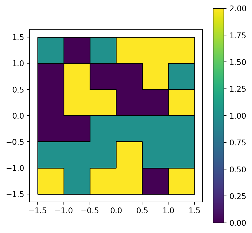
grain.tif converted to a polygon layer
As highlighted using edgecolor='black', neighboring pixels sharing the same raster value are dissolved into larger polygons. The rasterio.features.shapes function unfortunately does not offer a way to avoid this type of dissolving. One suggestion is to add unique values between 0 and 0.9999 to all pixels, convert to polygons, and then get back to the original values using np.floor.
5.5.2 Raster to points
To transform a raster to points, we can use the rasterio.transform.xy function. As the name suggests, the function accepts row and column indices, and transforms them into x- and y-coordinates (using the raster’s transformation matrix). For example, the coordinates of the top-left pixel can be calculated passing the (row,col) indices of (0,0).
src = rasterio.open('output/elev.tif')
rasterio.transform.xy(src.transform, 0, 0)
(np.float64(-1.25), np.float64(1.25))
Note
Keep in mind that the coordinates of the top-left pixel ((-1.25, 1.25)), as calculated in the above expression, refer to the pixel centroid. Therefore, they are not identical to the raster origin coordinates ((-1.5,1.5)), as specified in the transformation matrix, which are the coordinates of the top-left edge/corner of the raster (see Figure 5.9).
src.transformAffine(0.5, 0.0, -1.5,
0.0, -0.5, 1.5)To generalize the above expression to calculate the coordinates of all pixels, we first need to generate a grid of all possible row/column index combinations. This can be done using np.meshgrid, as follows.
height = src.shape[0]
width = src.shape[1]
cols, rows = np.meshgrid(np.arange(width), np.arange(height))
We now have two arrays, rows and cols, matching the shape of elev.tif and containing the corresponding row and column indices.
rowsarray([[0, 0, 0, 0, 0, 0],
[1, 1, 1, 1, 1, 1],
[2, 2, 2, 2, 2, 2],
[3, 3, 3, 3, 3, 3],
[4, 4, 4, 4, 4, 4],
[5, 5, 5, 5, 5, 5]])colsarray([[0, 1, 2, 3, 4, 5],
[0, 1, 2, 3, 4, 5],
[0, 1, 2, 3, 4, 5],
[0, 1, 2, 3, 4, 5],
[0, 1, 2, 3, 4, 5],
[0, 1, 2, 3, 4, 5]])These can be passed to rasterio.transform.xy to transform the indices into point coordinates, accordingly stored in lists of arrays x and y.
x, y = rasterio.transform.xy(src.transform, rows, cols)x[array([-1.25, -0.75, -0.25, 0.25, 0.75, 1.25]),
array([-1.25, -0.75, -0.25, 0.25, 0.75, 1.25]),
array([-1.25, -0.75, -0.25, 0.25, 0.75, 1.25]),
array([-1.25, -0.75, -0.25, 0.25, 0.75, 1.25]),
array([-1.25, -0.75, -0.25, 0.25, 0.75, 1.25]),
array([-1.25, -0.75, -0.25, 0.25, 0.75, 1.25])]y[array([1.25, 1.25, 1.25, 1.25, 1.25, 1.25]),
array([0.75, 0.75, 0.75, 0.75, 0.75, 0.75]),
array([0.25, 0.25, 0.25, 0.25, 0.25, 0.25]),
array([-0.25, -0.25, -0.25, -0.25, -0.25, -0.25]),
array([-0.75, -0.75, -0.75, -0.75, -0.75, -0.75]),
array([-1.25, -1.25, -1.25, -1.25, -1.25, -1.25])]Typically we want to work with the points in the form of a GeoDataFrame which also holds the attribute(s) value(s) as point attributes. To get there, we can transform the coordinates as well as any attributes to 1-dimensional arrays, and then use methods we are already familiar with (Section 1.2.6) to combine them into a GeoDataFrame.
x = np.array(x).flatten()
y = np.array(y).flatten()
z = src.read(1).flatten()
geom = gpd.points_from_xy(x, y, crs=src.crs)
pnt = gpd.GeoDataFrame(data={'value':z}, geometry=geom)
pnt| value | geometry | |
|---|---|---|
| 0 | 1 | POINT (-1.25 1.25) |
| 1 | 2 | POINT (-0.75 1.25) |
| 2 | 3 | POINT (-0.25 1.25) |
| ... | ... | ... |
| 33 | 34 | POINT (0.25 -1.25) |
| 34 | 35 | POINT (0.75 -1.25) |
| 35 | 36 | POINT (1.25 -1.25) |
36 rows × 2 columns
This ‘high-level’ workflow, like many other rasterio-based workflows covered in the book, is a commonly used one but lacking from the package itself. From the user’s perspective, it may be a good idea to wrap the workflow into a function (e.g., raster_to_points(src), returning a GeoDataFrame), to be re-used whenever we need it.
Figure 5.9 shows the input raster and the resulting point layer.
# Input raster
fig, ax = plt.subplots()
pnt.plot(column='value', legend=True, ax=ax)
rasterio.plot.show(src_elev, ax=ax);
# Points
fig, ax = plt.subplots()
pnt.plot(column='value', legend=True, edgecolor='black', ax=ax)
rasterio.plot.show(src_elev, alpha=0, ax=ax);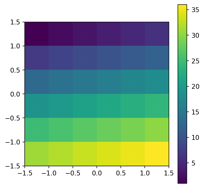
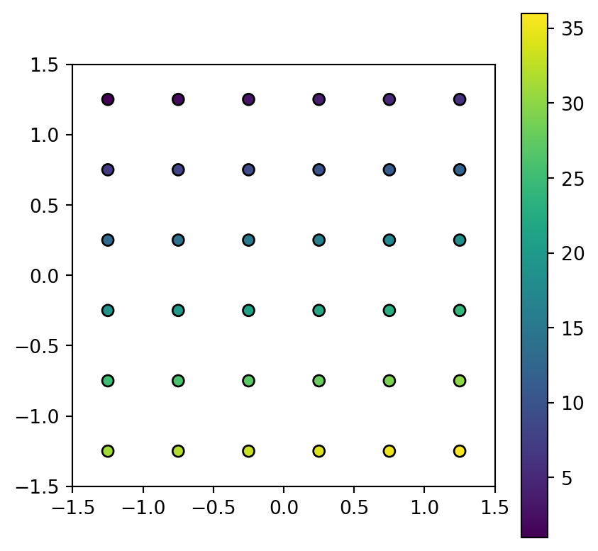
elev.tif
Note that ‘No Data’ pixels can be filtered out from the conversion, if necessary (see Section 5.6).
5.5.3 Raster to contours
Another common type of spatial vectorization is the creation of contour lines, representing lines of continuous height or temperatures (isotherms), for example. We will use a real-world digital elevation model (DEM) because the artificial raster elev.tif produces parallel lines (task for the reader: verify this and explain why this happens). Plotting contour lines is straightforward, using the contour=True option of rasterio.plot.show (Figure 5.10).
fig, ax = plt.subplots()
rasterio.plot.show(src_dem, ax=ax)
rasterio.plot.show(
    src_dem,
    ax=ax,
    contour=True,
    levels=np.arange(0,1200,50),
    colors='black'
);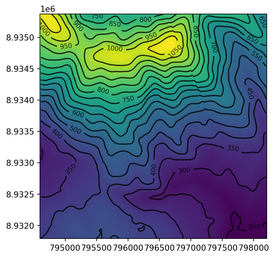
Unfortunately, rasterio does not provide any way of extracting the contour lines in the form of a vector layer, for uses other than plotting.
There are two possible workarounds:
- Using
gdal_contouron the command line (see below), or through its Python interface osgeo - Writing a custom function to export contour coordinates generated by, e.g., matplotlib or skimage
We demonstrate the first approach, using gdal_contour. Although we deviate from the Python-focused approach towards more direct interaction with GDAL, the benefit of gdal_contour is the proven algorithm, customized to spatial data, and with many relevant options. Both the gdal_contour program (along with other GDAL programs) and its osgeo Python wrapper, should already be installed on your system since GDAL is a dependency of rasterio. Using the command line pathway, generating 50 \(m\) contours of the dem.tif file can be done as follows.
os.system('gdal_contour -a elev data/dem.tif output/dem_contour.gpkg -i 50.0')Like all GDAL programs (also see gdaldem example in Section 3.3.4), gdal_contour works with files. Here, the input is the data/dem.tif file and the result is exported to the output/dem_contour.gpkg file.
To illustrate the result, let’s read the resulting dem_contour.gpkg layer back into the Python environment. Note that the layer contains an attribute named 'elev' (as specified using -a elev) with the contour elevation values.
contours1 = gpd.read_file('output/dem_contour.gpkg')
contours1| ID | elev | geometry | |
|---|---|---|---|
| 0 | 0 | 750.0 | LINESTRING (795382.355 8935384.... |
| 1 | 1 | 800.0 | LINESTRING (795237.703 8935384.... |
| 2 | 2 | 650.0 | LINESTRING (798098.379 8935384.... |
| ... | ... | ... | ... |
| 29 | 29 | 450.0 | LINESTRING (795324.083 8931774.... |
| 30 | 30 | 450.0 | LINESTRING (795488.616 8931774.... |
| 31 | 31 | 450.0 | LINESTRING (795717.42 8931774.8... |
32 rows × 3 columns
Figure 5.11 shows the input raster and the resulting contour layer.
fig, ax = plt.subplots()
rasterio.plot.show(src_dem, ax=ax)
contours1.plot(ax=ax, edgecolor='black');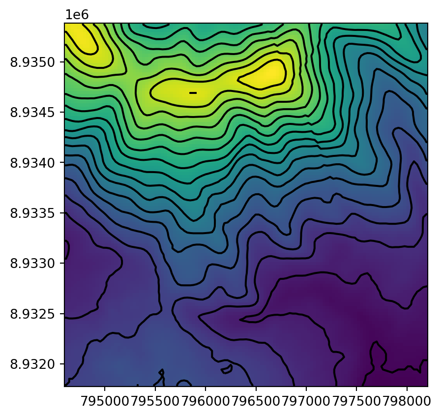
dem.tif raster, calculated using the gdal_contour program
5.6 Distance to nearest geometry
Calculating a raster of distances to the nearest geometry is an example of a ‘global’ raster operation (Section 3.3.6). To demonstrate it, suppose that we need to calculate a raster representing the distance to the nearest coast in New Zealand. This example also wraps many of the concepts introduced in this chapter and in previous chapters, such as raster aggregation (Section 4.3.2), raster conversion to points (Section 5.5.2), and rasterizing points (Section 5.4.1).
For the coastline, we will dissolve the New Zealand administrative division polygon layer and ‘extract’ the boundary as a 'MultiLineString' geometry (Figure 5.12). Note that .dissolve(by=None) (Section 2.2.2) calls .union_all on all geometries (i.e., aggregates everything into one group), which is what we want to do here.
coastline = nz.dissolve().to_crs(src_nz_elev.crs).boundary.iloc[0]
coastline
For a ‘template’ raster, we will aggregate the New Zealand DEM, in the nz_elev.tif file, to 5 times coarser resolution. The code section below follows the aggregation example in Section 4.3.2.
factor = 0.2
# Reading aggregated array
r = src_nz_elev.read(1,
    out_shape=(
        int(src_nz_elev.height * factor),
        int(src_nz_elev.width * factor)
        ),
    resampling=rasterio.enums.Resampling.average
)
# Updating the transform
new_transform = src_nz_elev.transform * src_nz_elev.transform.scale(
    (src_nz_elev.width / r.shape[1]),
    (src_nz_elev.height / r.shape[0])
)
The resulting array r/new_transform and the lines layer coastline are plotted in Figure 5.13. Note that the raster values are average elevations based on \(5 \times 5\) pixels, but this is irrelevant for the subsequent calculation; the raster is going to be used as a template, and all of its values will be replaced with distances to coastline (Figure 5.14).
fig, ax = plt.subplots()
rasterio.plot.show(r, transform=new_transform, ax=ax)
gpd.GeoSeries(coastline).plot(ax=ax, edgecolor='red');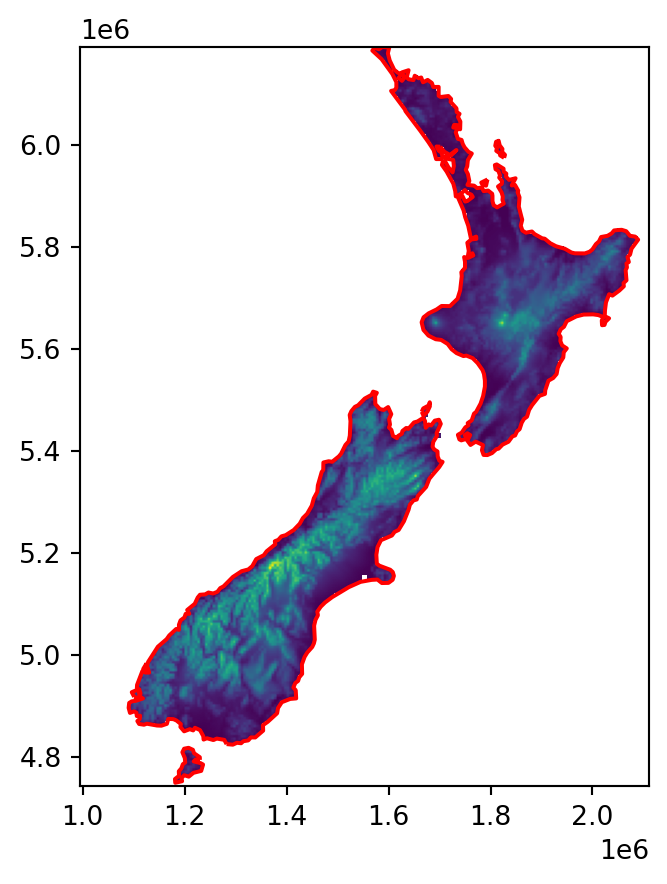
To calculate the actual distances, we must convert each pixel to a vector (point) geometry. For this purpose, we use the technique demonstrated in Section 5.5.2, but we’re keeping the points as a list of shapely geometries, rather than a GeoDataFrame, since such a list is sufficient for the subsequent calculation.
height = r.shape[0]
width = r.shape[1]
cols, rows = np.meshgrid(np.arange(width), np.arange(height))
x, y = rasterio.transform.xy(new_transform, rows, cols)
x = np.array(x).flatten()
y = np.array(y).flatten()
z = r.flatten()
x = x[~np.isnan(z)]
y = y[~np.isnan(z)]
geom = gpd.points_from_xy(x, y, crs=california.crs)
geom = list(geom)
geom[:5]
[<POINT (1572956.546 6189460.927)>,
<POINT (1577956.546 6189460.927)>,
<POINT (1582956.546 6189460.927)>,
<POINT (1587956.546 6189460.927)>,
<POINT (1592956.546 6189460.927)>]The result geom is a list of shapely geometries, representing raster cell centroids (excluding np.nan pixels, which were filtered out).
Now we can calculate the corresponding list of point geometries and associated distances, using the .distance method from shapely:
distances = [(i, i.distance(coastline)) for i in geom]
distances[0]
(<POINT (1572956.546 6189460.927)>, 826.7523956221047)Finally, we rasterize (see Section 5.4.1) the distances into our raster template.
image = rasterio.features.rasterize(
    distances,
    out_shape=r.shape,
    dtype=np.float64,
    transform=new_transform,
    fill=np.nan
)
image
array([[nan, nan, nan, ..., nan, nan, nan],
[nan, nan, nan, ..., nan, nan, nan],
[nan, nan, nan, ..., nan, nan, nan],
...,
[nan, nan, nan, ..., nan, nan, nan],
[nan, nan, nan, ..., nan, nan, nan],
[nan, nan, nan, ..., nan, nan, nan]])The final result, a raster of distances to the nearest coastline, is shown in Figure 5.14.
fig, ax = plt.subplots()
rasterio.plot.show(image, transform=new_transform, ax=ax)
gpd.GeoSeries(coastline).plot(ax=ax, edgecolor='red');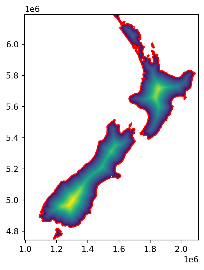
The answer is
src_srtm.meta['dtype'], which returns'uint16'.↩︎https://en.wikipedia.org/wiki/Bresenham%27s_line_algorithm↩︎